Blog

Introduction

If you are capable of reading this piece of text, it is certain that you have passed your infancy. As someone who has come a long way from infancy, did you ever think of how you LEARNED to stand-up, walk, and basically avoid the dangers? If you start to deeply analyze the whole phenomenon behind your journey, you will realize that you LEARNED FROM EXPERIENCE with every passing moment of your life. Isn’t it beautiful how the experience allowed you to be yourself, and explore the world to be where you are now?

Combined with the experience and the inputs acquired by the five senses, the human evolves through a journey of lifetime, while facing a vast array of successes, sorrows, challenges, and emotions. For instance, during your lifelong learning experience, if you are REWARDED for an action that you performed with goodwill, more often than not, you will be inclined to perform the same action at least few more times if it is guaranteed that you are rewarded for your actions. On the other hand, it is almost certain that you will end up restricting yourself from doing non-acceptable actions that heavily PENALIZE you. Irrespective of the task/action, this is a process that has inherently assisted us in making informed decisions based on the past experiences. Here, why do you think that we are we interested in the basic decision making process employed by the human? In this article, we will look into the possibilities of teaching the machines to mimic the experience-based human reasoning process, and we will show you a demonstration of how it is achieved in a methodical approach.

Analogy

Before diving into the technical aspects of the theory behind this approach, let us try to map our problem to a fundamental problem. Imagine that you are a baby who is stuck in a dark room, and you have no clue whatsoever on what you should do next. Since you are a baby, you do not have any idea about the surroundings, and unfortunately, you do not have anyone to ask for help. However, you have the option of taking baby steps forward or right or backward or left. At the same time, suppose that you have a stock of chocolate (100 g) in your hand, and you really love them. Well, who doesn’t? Nonetheless, you can see light waves coming towards you from the other side of the room (possibly a way to get out of darkness). Gradually, you take random steps, and to your surprise, you realize that the stock of your chocolate changes depending on the actions you take, as follows.

• Whenever you touch a wall of the dark room, you lose 20 g of chocolate.
• For each baby step taken by you, if it gets you closer to the light waves, your chocolate stock gets increased by 2 g. If you move away from the light waves, you are penalized by taking 10 g of chocolate away from you.
• If you somehow manage to reach the source of light waves, you are given 100 g of chocolate.

Since the baby loves chocolates, the baby begins realizing the pattern that benefits him/her more and the baby eventually reaches the source of light waves. This is an interesting analogy to imply how the baby’s brain picks the more rewarding patterns while avoiding patterns that negatively impact the baby.

While it is tempting to understand how a human picks such patterns, what would you say if we can convince you that the computer is also capable of mimicking the human behaviour in terms of self learning and pattern recognition? Reinforcement Learning is an interesting research area that allows us to achieve the task of making computers recognize such patterns, and with this article, it is expected to bring you an understanding of how it can be achieved.

Reinforcement Learning

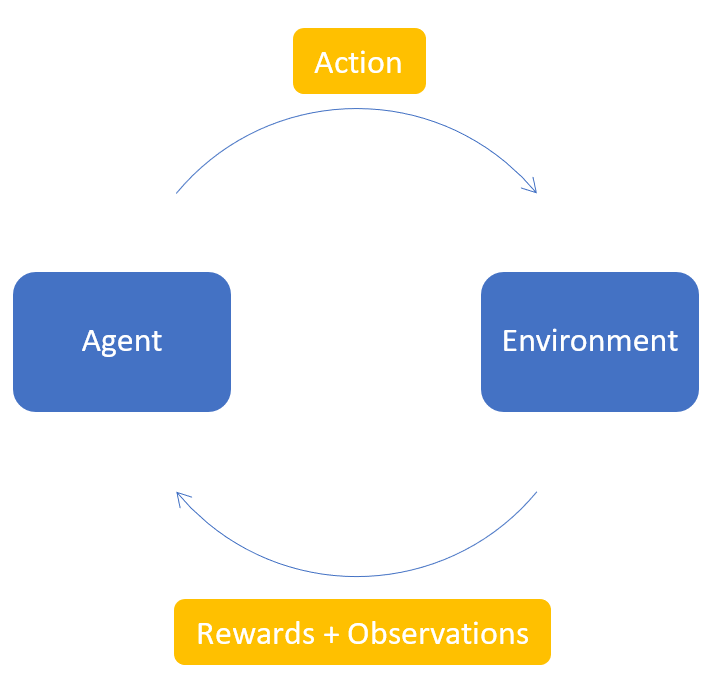
Reinforcement Learning (RL) focuses on teaching agents through trial and error. It learns by actively engaging with an environment. It consists of four fundamental concepts that make up as the building blocks of Reinforcement Learning.

• Agent: The entity (actor) that operates in the environment according to a policy
• Environment: The world in which the agent operates in
• Action: The possible action done by the agent
• Rewards: The points received by the agent upon performing an action, based on its actions on the environment.
• Observations: The observations available after performing the action

If we can consider and compare the analogy explained previously with the concepts of Reinforcement Learning, the following mapping can be illustrated.

Agent	↔︎	Baby
Environment	↔︎	The Dark Room
Action	↔︎	Forwards, Right, Backwards, Left
Rewards	↔︎	Chocolates
Observations	↔︎	Baby realizing what happened after performing an action

Reinforcement Learning behaves as the foundation for our goal, and the concepts of Q-Learning and Deep Q-Learning can be employed as aids to implement the solution. In the following sections, the concepts behind Q-Learning and Deep Q-Learning are briefly explained.

Q-Learning

As explained previously, the reward awarded for each action at each step is a known element within our framework. The agent is supposed to carry out a sequence of actions to maximize the total reward where the total reward can be termed as the Q-value. The Q-value can be obtained as follows.

Q(s,a) = r(s,a) + γ max Q (s',a)

In the formula, the Q value for performing the action a at state s is obtained by considering the existing reward [r(s,a)] and the highest possible Q-value obtainable from the state s' (next state). In this equation, γ (Gamma) is the discount factor which determines the contribution of the future rewards.

Since this acts as a recursive function, Q(s’,a) depends on Q(s”,a) and we essentially get a recursive function. As such, we initialize the model by initializing a Q value, and then let the agent choose a suitable action. The chosen action could be a predicted action or a random action if the agent is at the early stages of training. Based on the chosen action, the action is performed and its reward is measured before updating the Q value. This sequence of steps (except the initialization of Q value) is repeated during the training process.

Deep Q-Learning

The combination of Q-Learning and Deep Learning enables us to utilize Deep Q-Learning where we finally get a neural network for taking the optimum actions. While the usual Q-Learning can be used for simple tasks, it can be infeasible in occasions where we have a large number of states along with a big action space. This is where the concepts of neural networks become handy as it allows the agent to approximate the values of the Q-learning function. In this neural network, we utilize the Mean Squared Error as our loss function, which can be illustrated as follows.

loss = (Qnew - Q)^2 where the Q values can be obtained using the Bellman’s equation given above.

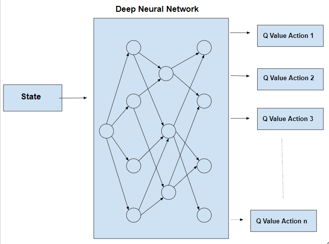
In the above neural network, we choose the action that corresponds to the maximum Q value among the n number of actions given as the output. More information regarding how these theorems are applied to our use case, are given in the subsequent sections.

Implementation of Analogy

For the sake of simplicity, we will create a simple 2D game that can represent the previously explained analogy where both the baby and the light wave sources are represented by squares (different colours). The game is encapsulated by four walls (borders of the 2D game), and the baby is rewarded or penalized based on the actions taken. On the other hand, if the baby somehow manages to reach the light source, the baby is heavily rewarded. The entire game is presented to the audience as if the audience is watching the game from an aerial view as it provides the best possible view to understand the course of actions.

In the meantime, we will also mention a score that the baby can accumulate over different episodes within the game. If the baby manages to reach the light source, the light source will be randomly placed somewhere else within the room, and the baby will have to go to the new position of the light source. The game scoring rules will be as follows.

• Baby can take the following actions where the baby will move by a unit distance on the given direction.
  • Forward
  • Backward
  • Left
  • Right
• Baby takes a step:
  • If the step results in baby getting closer to the light source → +1 point
  • If the step results in baby getting away from the light source → -5 points
• If baby reaches the light source → +50 points (light source will get placed at a different location after obtaining +50 points)
• If baby hits one of the walls → Game Over

Based on the defined game rules and the expected goal, it is expected to implement the game as shown in the following sketch.

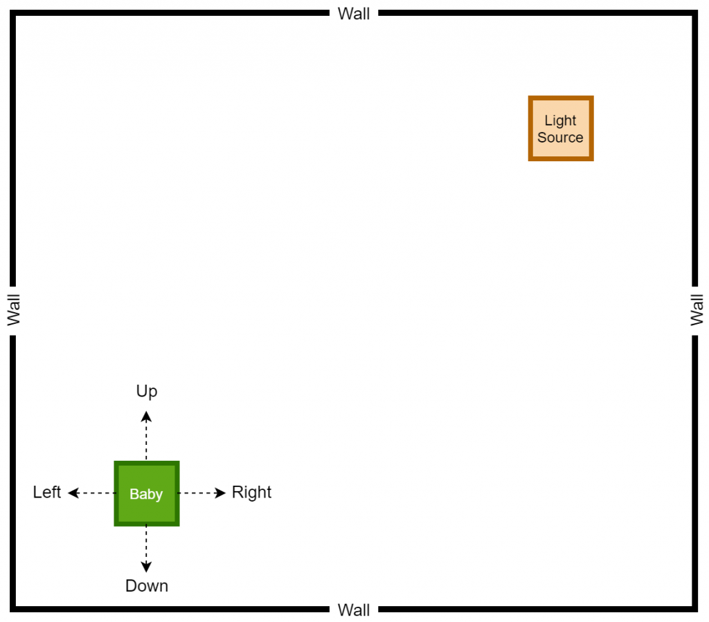
The Up, Right, Down, and Left arrows represent the actions that can be performed by the baby, and the corresponding directions are assigned by assuming that the game is controlled from an aerial position. As it stands, our goal is to teach the baby to take the correct actions to reach the light source, and it is performed by rewarding or penalizing the baby based on the actions taken by the baby himself/herself.

We will first attempt to create a game that can be played by a human where the keyboard controls can be used to control the actions taken by the baby. Afterwards, we will work on creating a computer agent along with a deep learning model that can effectively mimic the human behaviour to eventually automate the actions taken by the baby.

The Game

The game will be implemented by considering Python as the programming language, and we also employ the services of a Python 2D game library known as PyGame. As usually, it is required to utilize a Python environment for the purpose of creating this game, and we encourage you to install the PyGame library as a prerequisite.

Game (Played by a human)

Once the prerequisites are satisfied, we implemented the human-playable game where the code is self-explanatory with the given comments.

game.py

import pygame
import random
from enum import Enum
from collections import namedtuple
import math

pygame.init()

font = pygame.font.Font('arial.ttf', 25)

# Possible directions of the Baby
class Direction(Enum):
    RIGHT = 1
    LEFT = 2
    UP = 3
    DOWN = 4

Point = namedtuple('Point', 'x, y')

#RGB Colours
WHITE = (255, 255, 255)
BLACK = (0, 0, 0)
GREEN1 = (107,142,35)
GREEN2 = (173,255,47)

BLOCK_SIZE = 20
SPEED = 3
NEGATIVE_SCORE_THRESHOLD = 20

class Baby():

    def __init__(self, w = 640, h = 480):
        self.w = w
        self.h = h

        # Initialize the Display
        self.display = pygame.display.set_mode((self.w, self.h))
        pygame.display.set_caption('Path Finder')
        self.clock = pygame.time.Clock()

        # Initialize the game state and place the target
        self.direction = Direction.LEFT
        self.head = Point(self.w/2, self.h/2)
        self.head_prev = Point(self.w/2, self.h/2)

        self.score = 0
        self.target = None

        self._place_target()

    def _place_target(self):
        # Place the target inside the window
        x = random.randint(0, (self.w - BLOCK_SIZE) // BLOCK_SIZE) * BLOCK_SIZE
        y = random.randint(0, (self.h - BLOCK_SIZE) // BLOCK_SIZE) * BLOCK_SIZE
        self.target = Point(x, y)

        # To ensure that the target does not get placed on the Baby
        if self.target == self.head:
            self._place_target()

    def play_step(self):

        # Collect user input
        for event in pygame.event.get():
            if event.type == pygame.QUIT:
                pygame.quit()
                quit()

            if event.type == pygame.KEYDOWN:
                if event.key == pygame.K_LEFT:
                    self.direction = Direction.LEFT
                elif event.key == pygame.K_RIGHT:
                    self.direction = Direction.RIGHT
                elif event.key == pygame.K_UP:
                    self.direction = Direction.UP
                elif event.key == pygame.K_DOWN:
                    self.direction = Direction.DOWN

        # Move the Baby
        self._move(self.direction)  # Update the head

        # Check if the game is over
        game_over = False
        if self._is_collision() or self.score < -NEGATIVE_SCORE_THRESHOLD:
            game_over = True
            return game_over, self.score

        # If the Baby is moving away, penalize
        if self._is_moving_away():
            self.score -= 5

        # If the Baby is getting close, reward
        if self._is_moving_close():
            self.score += 1

        # Place new target or move the Baby
        if self.head == self.target:
            self.score += 10
            self._place_target()

        # Update UI and clock
        self._update_ui()
        self.clock.tick(SPEED)

        # Return if the game is over and score
        return game_over, self.score

    def _is_collision(self):
        # Does it hit the boundary?
        if (self.head.x > self.w - BLOCK_SIZE) or (self.head.x < 0) or (self.head.y > self.h - BLOCK_SIZE) or (self.head.y < 0):
            return True                  
        return False

    def _is_moving_away(self):
        prev_distance = math.hypot(self.head_prev.x - self.target.x, self.head_prev.y - self.target.y)
        current_distance = math.hypot(self.head.x - self.target.x, self.head.y - self.target.y)   
        if current_distance > prev_distance:
            return True          
        return False

    def _is_moving_close(self):
        prev_distance = math.hypot(self.head_prev.x - self.target.x, self.head_prev.y - self.target.y)
        current_distance = math.hypot(self.head.x - self.target.x, self.head.y - self.target.y)    
        if current_distance > prev_distance:
            return False  
        return True

    def _move(self, direction):
        x = self.head.x
        y = self.head.y
        self.head_prev = Point(x, y)

        if direction == Direction.RIGHT:
            x += BLOCK_SIZE
        elif direction == Direction.LEFT:
            x -= BLOCK_SIZE     
        elif direction == Direction.DOWN:
            y += BLOCK_SIZE  
        elif direction == Direction.UP:
            y -= BLOCK_SIZE  

        self.head = Point(x, y)

    def _update_ui(self):
        self.display.fill(BLACK)

        # Drawing the Baby
        pygame.draw.rect(self.display, GREEN1, pygame.Rect(self.head.x, self.head.y, BLOCK_SIZE, BLOCK_SIZE))
        pygame.draw.rect(self.display, GREEN2, pygame.Rect(self.head.x + 4, self.head.y + 4, 12, 12))

        # Drawing the Target
        pygame.draw.rect(self.display, WHITE, pygame.Rect(self.target.x, self.target.y, BLOCK_SIZE, BLOCK_SIZE))

        text = font.render("Score: " + str(self.score), True, WHITE)
        self.display.blit(text, [0, 0])
        pygame.display.flip()

if __name__ == '__main__':
    game = Baby()

    # Game Loop
    while True:
        game_over, score = game.play_step()
        
        # Break if the game is over
        if game_over == True:
            break

    print('Final Score: ', score)

    pygame.quit()

Next, we create an agent that can effectively make the computer learn by playing the game. However, it is also important to initialize a deep learning model that gets trained based on the actions performed by the agent.

Reward Function

The reward function plays a critical role in making the computer learn all the “Good” and “Bad” actions that it can learn. For instance, our goal is to positively reward for all the good actions and to negatively reward for bad actions. At the same time, we have attempted to quantify the “goodness” and “badness”, as it gives the computer a degree of freedom in learning.

As shown in the following pseudocode, the baby is rewarded negatively for each move that results in a collision with one of the four walls. Similarly, if the baby is trying to move away from the light source, for each move that results in an away movement, the baby is rewarded negatively. It should be noted that the collision avoidance has a higher priority, and as a result, the negative reward for collision avoidance has a higher magnitude compared to away movement. In a similar manner, the baby is positively rewarded for getting close to the light source, and for reaching the target.

reward = 0
game_over = False

if (baby collides with a wall):
    game_over = True
    reward = -10

# If the baby is moving away, penalize by rewarding negatively.
if (baby moves away from the light source):
    reward = -5

# The baby must be rewarded for attempting to get close to the target.
if (baby gets close to the light source):
    reward = 5

# If the baby reaches the target, baby must be rewarded accordingly.
if (baby reaches light source):
    reward += 10

In the following code blocks, the behaviour of both the agent and the model are demonstrated.

Agent

The agent takes care of the task of training the baby to identify the patterns and eventually learn what affects the baby most. The agent utilizes both the game environment and the created model to handle and coordinate the sequences of actions within the game. As shown in the code itself, the agent creates two objects, one from the game environment and the other one from the model. Further, some of the model hyperparameters are also set by the agent, and such hyperparameters are provides as inputs during the model creation time.

agent.py

import torch
import random
import numpy as np
from collections import deque
from game import BabyRL, Direction, Point
from model import Linear_QNet, QTrainer
from helper import plot

MAX_MEMORY = 100_000
BATCH_SIZE = 1000
LR = 0.001

class Agent:

    def __init__(self):
        self.n_games = 0

        # Indicates the Randomness
        self.epsilon = 0

        # Indicates the Discount Rate
        self.gamma = 0.9

        # Once the program reaches the maxlen, it will pop elements from the left side of the deque data structure
        self.memory = deque(maxlen=MAX_MEMORY)

        self.model = Linear_QNet(8,256,4)
        self.trainer = QTrainer(self.model, lr = LR, gamma = self.gamma)

    def get_state(self, game):
        dir_u = game.direction == Direction.UP
        dir_r = game.direction == Direction.RIGHT
        dir_d = game.direction == Direction.DOWN
        dir_l = game.direction == Direction.LEFT

        state = [
            # Moving Direction
            dir_u,
            dir_r,
            dir_d,
            dir_l,

            # Target Location
            game.target.x < game.head.x, # Target - Left
            game.target.x > game.head.x, # Target - Right
            game.target.y < game.head.y, # Target - Up
            game.target.y > game.head.y  # Target - Down 
        ]

        return np.array(state, dtype=int)

    def remember(self, state, action, reward, next_state, done):
        # Append as a single element
        self.memory.append((state, action, reward, next_state, done))

    def train_long_memory(self):
        # Sample into batches only if the length of elements exceed the BATCH_SIZE
        if len(self.memory) > BATCH_SIZE:
            mini_sample = random.sample(self.memory, BATCH_SIZE) # List of tuples 
        else:
            mini_sample = self.memory

        # Forming individual arrays for each variable - Alternatively, you may use a for-loop for achieving this task.
        states, actions, rewards, next_states, dones = zip(*mini_sample)
        self.trainer.train_step(states, actions, rewards, next_states, dones)

    def train_short_memory(self, state, action, reward, next_state, done):
        self.trainer.train_step(state, action, reward, next_state, done)

    def get_action(self, state):
        # Random Actions: Tradeoff between Exploration and Exploitation
        self.epsilon = 80 - self.n_games
        final_action = [0, 0, 0, 0]
        if random.randint(0, 200) < self.epsilon:
            action = random.randint(0, 3)
            final_action[action] = 1
        else:
            state0 = torch.tensor(state, dtype=torch.float)
            prediction = self.model(state0)
            action = torch.argmax(prediction).item()
            final_action[action] = 1

        return final_action


def train():
    plot_scores = []
    plot_mean_scores = []
    total_score = 0
    record = -50
    agent = Agent()
    game = BabyRL()

    while True:
        # Get the old state
        state_old = agent.get_state(game)

        # Determine the action based on the old state
        computed_action = agent.get_action(state_old)

        # Perform the action and get the new state
        reward, done, score = game.play_step(computed_action)
        state_new = agent.get_state(game)

        # Train short memory
        agent.train_short_memory(state_old, computed_action, reward, state_new, done)

        # Remember
        agent.remember(state_old, computed_action, reward, state_new, done)

        if done:
            # The game is over, and it needs to be reset. A new game needs to be started, thus the number of games increases.
            game.reset()
            agent.n_games += 1

            # Train long memory
            agent.train_long_memory()

            # Save each model after a defined number of iterations
            if agent.n_games % 5 == 0:
                agent.model.save(agent.n_games)

            # If we have a new record score, update it and save the model for reusability
            if score > record:
                record = score
                agent.model.save(agent.n_games, best = True)

            print("Game #: ", agent.n_games, ", Score: ", score, ", Record Score: ", record)

            # Plotting to be done below
            plot_scores.append(score)
            total_score += score
            mean_score = total_score / agent.n_games
            plot_mean_scores.append(mean_score)
            plot(plot_scores, plot_mean_scores, agent.n_games)
 
if __name__ == '__main__':
    train()

Model

As explained previously, we utilize Deep Q-Learning as the backbone of our model, and the responsibility of the model is to inform the baby of the correct decision that must be made after each move. In other words, the model acts as the brain of the child, as the model helps the baby in making the critical decisions to eventually reach the target while avoiding the obstacles.

Inputs

The inputs to the model are provided as a vector of binary values to represent the following states.

• X1 - Whether the baby moves towards the top direction
• X2 - Whether the baby moves towards the right direction
• X3 - Whether the baby moves towards the bottom direction
• X4 - Whether the baby moves towards the left direction
• X5 - Whether the light source is to the top of baby
• X6 - Whether the light source is to the right of baby
• X7 - Whether the light source is to the bottom of baby
• X8 - Whether the light source is to the left of baby

Based on the input values, a vector of inputs is created as follows.

[X1, X2, X3, X4, X5, X6, X7, X8]

Architecture

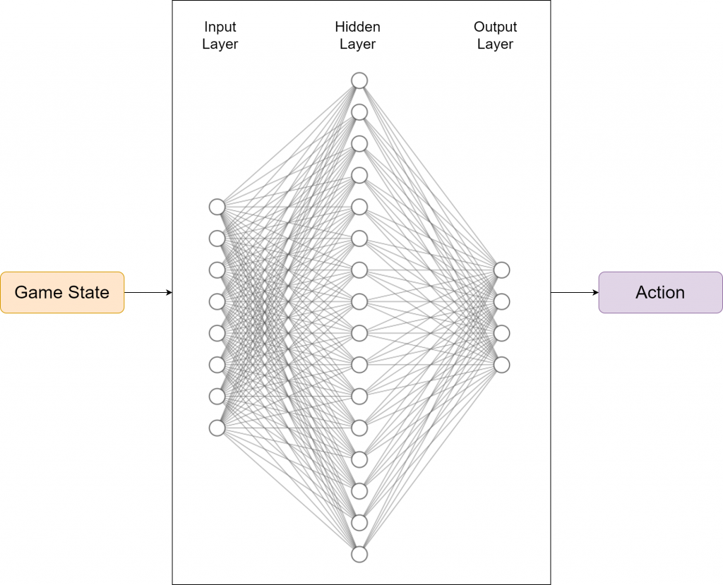
For the model, we have utilized the input layer, a single hidden layer with 256 neurons, and finally an output layer to release the actions. ReLu is used as the activation function between the layers, and in future iterations, the deeper models will be tested to see how effective the model will be. In terms of the choice of the optimizer, while we have a number of choices, we decided to make use of Adam optimizer as it has found to be effective in most of the scenarios. On the other hand, we consider the Mean Squared Error (MSE) as the evaluation criteria, as we continuously attempt to minimize the MSE. The model requires several hyperparameters, and we have used the following hyperparameter values to start with: Learning Rate = 0.001, Batch Size = 1000, and Gamma = 0.9.

Outputs

The output defines the correct action that must be taken by the baby in order to maximize the benefits obtained by the baby. As such, the output represents the action space along with their probabilities that correspond to the maximization of rewards. An example is as follows.

[Q value for Top Move, Q value for Right Move, Q value for Bottom Move, Q value for Left Move]

Among the output Q values, the action with the highest Q value is chosen, and the action is accordingly taken by the baby.

Implementation

Based on the parameters given above, the neural network can be illustrated as follows. In this particular problem, we have 256 neurons in the hidden layer whereas the neurons corresponding to the input layer and output layer, are illustrated based on actual values.

The following file demonstrates the implementation of the model, using PyTorch.
model.py

import torch
import torch.nn as nn
import torch.optim as optim
import torch.nn.functional as F
import os
from datetime import datetime

VERSION = 1

class Linear_QNet(nn.Module):
    def __init__(self, input_size, hidden_size, output_size):
        super().__init__()
        self.linear1 = nn.Linear(input_size, hidden_size)
        self.linear2 = nn.Linear(hidden_size, output_size)

    def forward(self, x):
        x = F.relu(self.linear1(x))
        x = self.linear2(x)
        return x

    def save(self, n_games, best = False):
        model_folder_path = './model/v' + str(VERSION)
        date = datetime.today().strftime('%Y-%m-%d')
        if not os.path.exists(model_folder_path):
            os.makedirs(model_folder_path)
        if best:
            file_name = os.path.join(model_folder_path, 'best_' + str(date) + '_' + str(n_games) + '.pth')
        else:           
            file_name = os.path.join(model_folder_path, str(date) + '_' + str(n_games) + '.pth')
        torch.save(self.state_dict(), file_name)

    def load(self, file_name = 'model.pth'):
        model_folder_path = './model'
        file_name = os.path.join(model_folder_path, file_name)

        if os.path.isfile(file_name):
            self.load_state_dict(torch.load(file_name))
            self.eval()
            print ('Loading existing state dict.')
            return True
        
        print ('No existing state dict found. Starting from scratch.')
        return False


class QTrainer:
    def __init__(self, model, lr, gamma):
        self.model = model
        self.lr = lr
        self.gamma = gamma
        self.optimizer = optim.Adam(model.parameters(), lr = self.lr)
        self.criterion = nn.MSELoss()

    def train_step(self, state, action, reward, next_state, done):
        state = torch.tensor(state, dtype=torch.float)
        next_state = torch.tensor(next_state, dtype=torch.float)
        action = torch.tensor(action, dtype=torch.long)
        reward = torch.tensor(reward, dtype=torch.float)

        if len(state.shape) == 1:
            # x > (1, x)
            state = torch.unsqueeze(state, 0) # Axis 0
            next_state = torch.unsqueeze(next_state, 0) # Axis 0
            action = torch.unsqueeze(action, 0) # Axis 0
            reward = torch.unsqueeze(reward, 0) # Axis 0
            done = (done, )

        # 1: Predicted Q values with the current state
        pred = self.model(state)

        target = pred.clone()
        for idx in range(len(done)):
            Q_new = reward[idx]
            if not done[idx]:
                # 2: Q_new = r + y * max(next_predicted_Q_value) -> Do this only if not done
                Q_new = reward[idx] + self.gamma * torch.max(self.model(next_state[idx]))
            target[idx][torch.argmax(action[idx]).item()] = Q_new

        self.optimizer.zero_grad()
        loss = self.criterion(target, pred)
        loss.backward()

        self.optimizer.step()

Game (Played by an Agent)

In order to accommodate the addition of Agent and Model, the game.py needs to be modified as shown below.

game.py

import pygame
import random
from enum import Enum
from collections import namedtuple
import math
import numpy as np

pygame.init()

font = pygame.font.Font('arial.ttf', 25)

# Possible directions of the Baby
class Direction(Enum):
    RIGHT = 1
    LEFT = 2
    UP = 3
    DOWN = 4

Point = namedtuple('Point', 'x, y')

#RGB Colours
WHITE = (255, 255, 255)
BLACK = (0, 0, 0)
GREEN1 = (107,142,35)
GREEN2 = (173,255,47)

BLOCK_SIZE = 30
SPEED = 60
NEGATIVE_SCORE_THRESHOLD = 30

class BabyRL():

    def __init__(self, w = 960, h = 720):
        self.w = w
        self.h = h

        # Initialize the Display
        self.display = pygame.display.set_mode((self.w, self.h))
        pygame.display.set_caption('Path Finder')
        self.clock = pygame.time.Clock()
        self.reset()

    def reset(self):
        # Initialize the game state and place the target
        self.direction = Direction.LEFT
        self.head = Point(self.w/2, self.h/2)
        self.head_prev = Point(self.w/2, self.h/2)

        self.score = 0
        self.target = None

        self._place_target()
        self.frame_iteration = 0

    def _place_target(self):
        # Place the target inside the window
        x = random.randint(0, (self.w - BLOCK_SIZE) // BLOCK_SIZE) * BLOCK_SIZE
        y = random.randint(0, (self.h - BLOCK_SIZE) // BLOCK_SIZE) * BLOCK_SIZE
        self.target = Point(x, y)

        # To ensure that the target does not get placed on the Baby
        if self.target == self.head:
            self._place_target()

    def play_step(self, action):
        
        # For each play_step, the number of frames must be iterated.
        self.frame_iteration += 1

        # Collect user input to catch the QUIT event. Unlike the game played by humans, we do not capture KEYDOWN inputs for determining the direction.
        # Instead, the computer must decide which action to take. As such, the "action" is a parameter of the play_step function.
        for event in pygame.event.get():
            if event.type == pygame.QUIT:
                pygame.quit()
                quit()

        # Move the Baby based on the "action" determined by the computer.
        # Previously, we used self.direction, which was determined by the human player.
        self._move(action)  # Update the head

        # Check if the game is over
        # If the game is over, a negative reward must be awarded to discourage the events of game over.
        reward = 0
        game_over = False
        if self.is_collision() or self.score < -NEGATIVE_SCORE_THRESHOLD:
            game_over = True
            reward = -10
            game_over_text = font.render("GAME OVER!", True, WHITE)
            game_over_text_rect = game_over_text.get_rect(center=(self.w/2, self.h/2))
            self.display.blit(game_over_text, game_over_text_rect)
            pygame.display.flip()
            return reward, game_over, self.score

        # If the Baby is moving away, penalize by deducting the score.
        if self._is_moving_away():
            self.score -= 5

        # If the Baby is getting close, award more scores. 
        # Further, the Baby must be rewarded for attempting to get clos to the target.
        if self._is_moving_close():
            self.score += 1
            reward += 1

        # Place new target or move the Baby
        # If the Baby reaches the target, it must be rewarded accordingly.
        if self.head == self.target:
            self.score += 10
            reward += 10
            self._place_target()

        # Update UI and clock
        self._update_ui()
        self.clock.tick(SPEED)

        # Return if the game is over and score
        return reward, game_over, self.score

    def is_collision(self):
        # Does it hit the boundary?
        if (self.head.x > self.w - BLOCK_SIZE) or (self.head.x < 0) or (self.head.y > self.h - BLOCK_SIZE) or (self.head.y < 0):
            return True                  
        return False

    def _is_moving_away(self):
        prev_distance = math.hypot(self.head_prev.x - self.target.x, self.head_prev.y - self.target.y)
        current_distance = math.hypot(self.head.x - self.target.x, self.head.y - self.target.y)   
        if current_distance > prev_distance:
            return True          
        return False

    def _is_moving_close(self):
        prev_distance = math.hypot(self.head_prev.x - self.target.x, self.head_prev.y - self.target.y)
        current_distance = math.hypot(self.head.x - self.target.x, self.head.y - self.target.y)    
        if current_distance > prev_distance:
            return False  
        return True

    def _move(self, action):
        # [Up, Right, Down, Left]

        if np.array_equal(action, [1, 0, 0, 0]):
            new_direction = Direction.UP
        elif np.array_equal(action, [0, 1, 0, 0]):
            new_direction = Direction.RIGHT
        elif np.array_equal(action, [0, 0, 1, 0]):
            new_direction = Direction.DOWN
        elif np.array_equal(action, [0, 0, 0, 1]):
            new_direction = Direction.LEFT

        self.direction = new_direction

        x = self.head.x
        y = self.head.y
        self.head_prev = Point(x, y)

        if self.direction == Direction.RIGHT:
            x += BLOCK_SIZE
        elif self.direction == Direction.LEFT:
            x -= BLOCK_SIZE     
        elif self.direction == Direction.DOWN:
            y += BLOCK_SIZE  
        elif self.direction == Direction.UP:
            y -= BLOCK_SIZE  

        self.head = Point(x, y)

    def _update_ui(self):
        self.display.fill(BLACK)

        # Drawing the Baby
        pygame.draw.rect(self.display, GREEN1, pygame.Rect(self.head.x, self.head.y, BLOCK_SIZE, BLOCK_SIZE))
        pygame.draw.rect(self.display, GREEN2, pygame.Rect(self.head.x + 6, self.head.y + 6, 18, 18))

        # Drawing the Target
        pygame.draw.rect(self.display, WHITE, pygame.Rect(self.target.x, self.target.y, BLOCK_SIZE, BLOCK_SIZE))

        text = font.render("Score: " + str(self.score), True, WHITE)
        self.display.blit(text, [0, 0])
        pygame.display.flip()

Now you have a game where the computer learns gradually to reach the target.

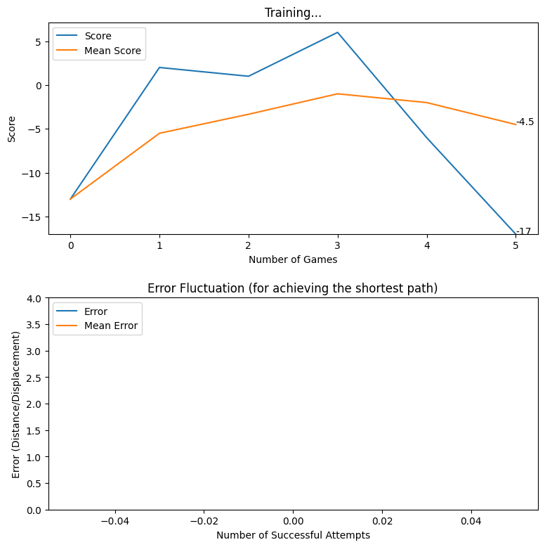
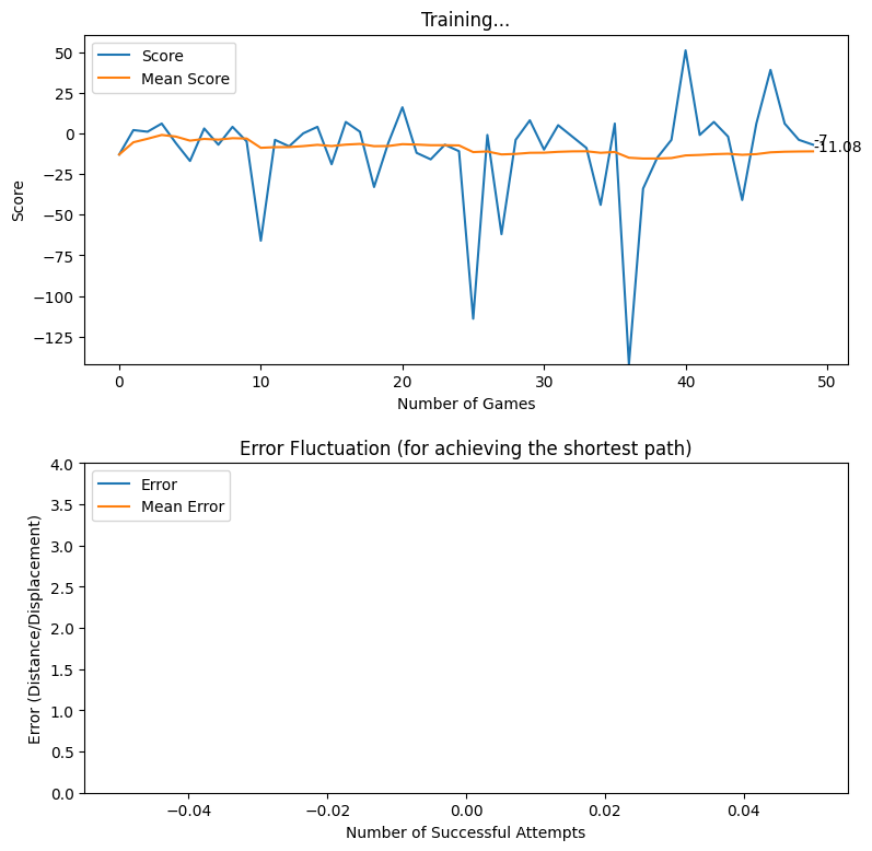
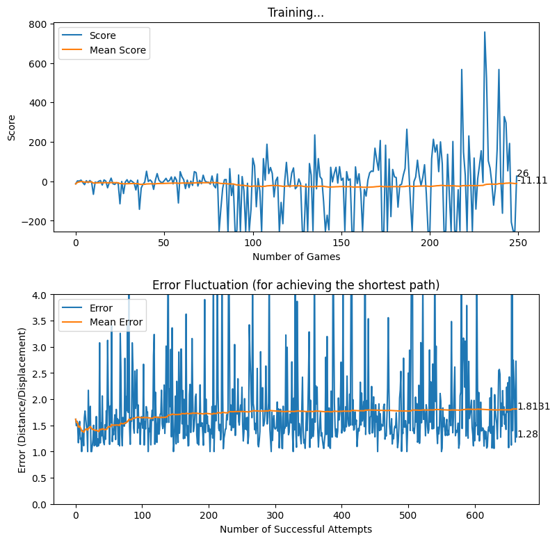
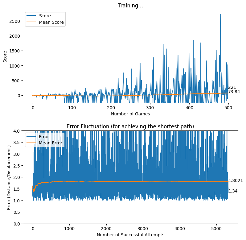
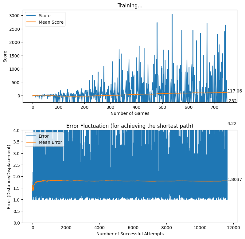
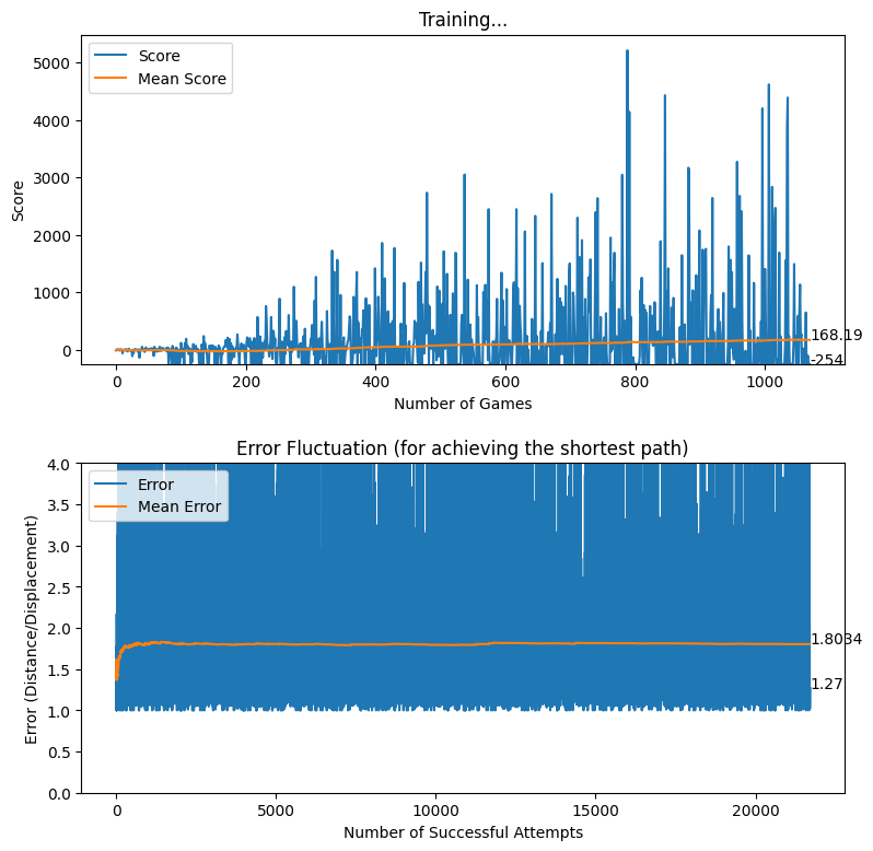
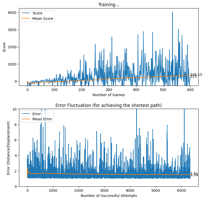
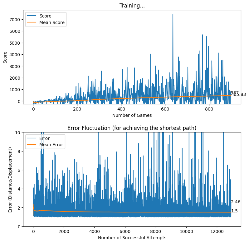
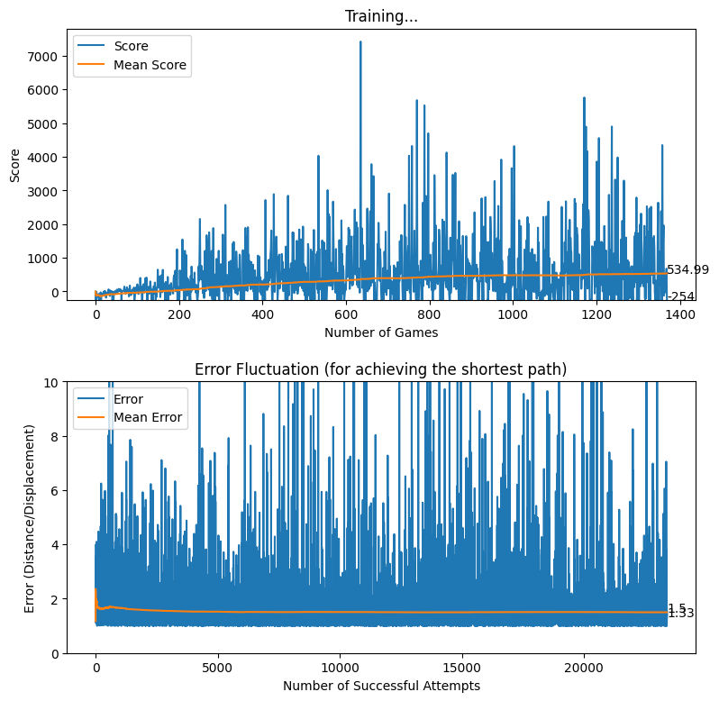
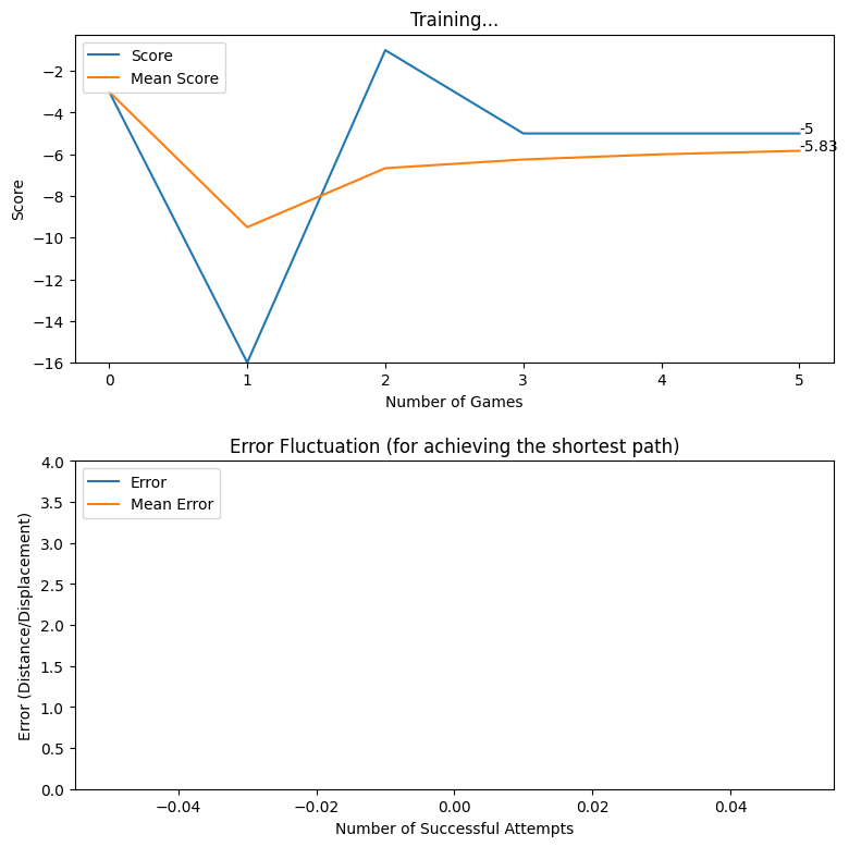
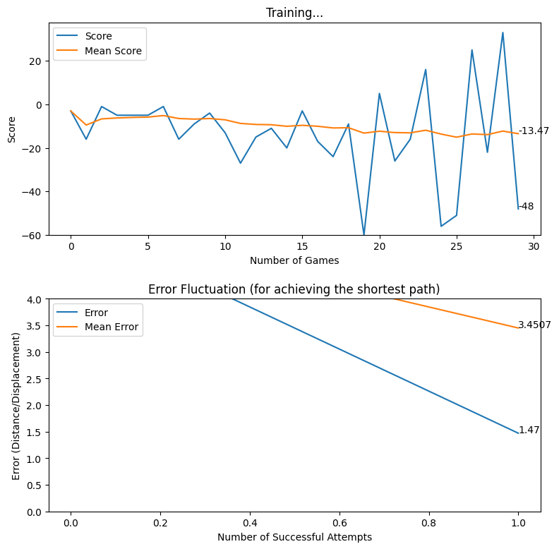
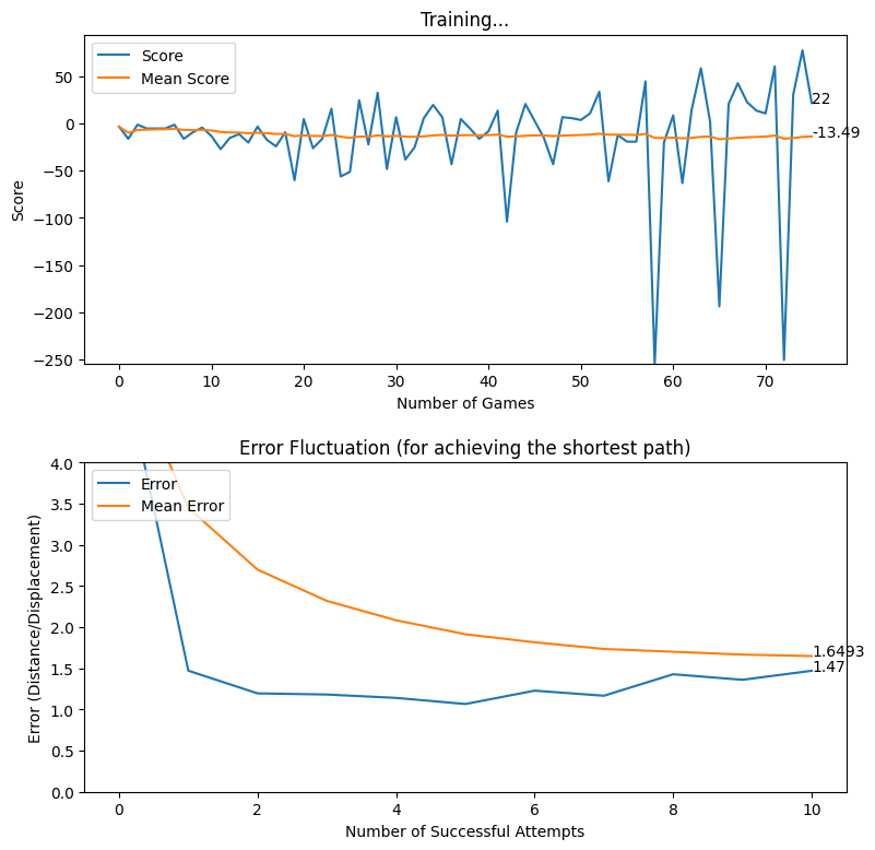
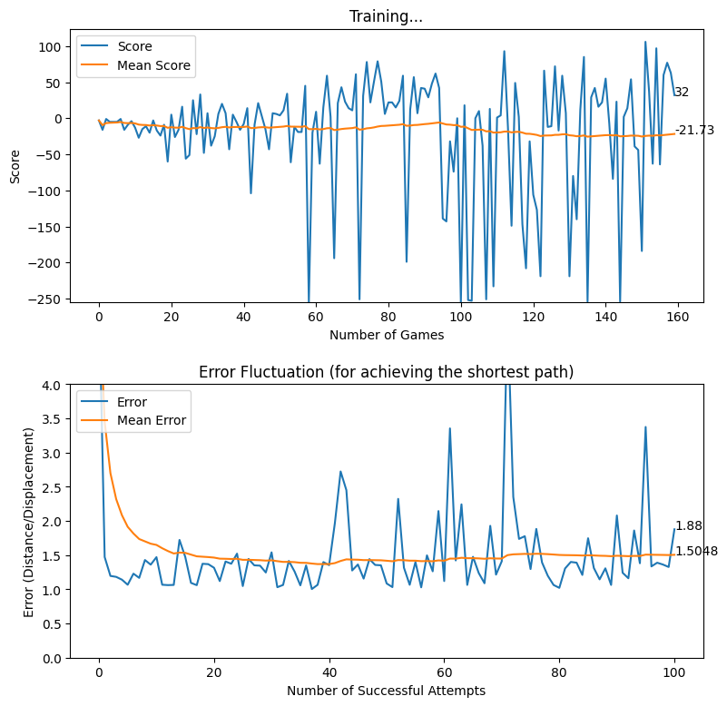
Demonstration

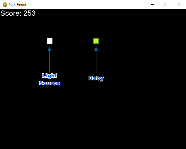
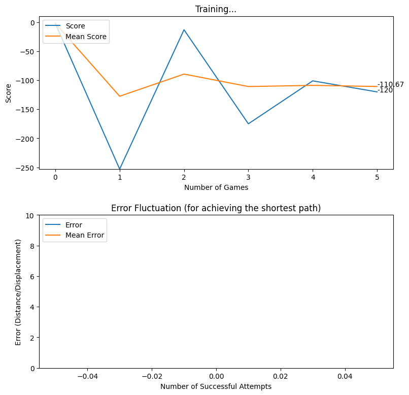
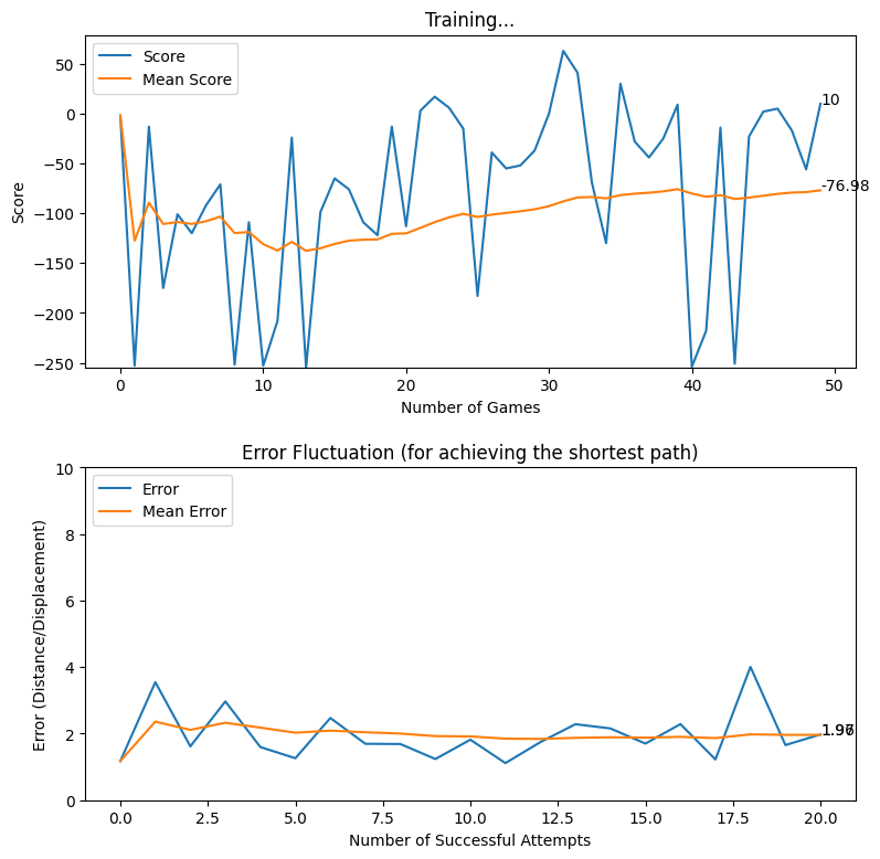
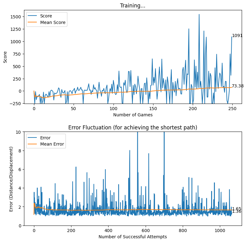
After creating the game as explained in the previous sections, we actually trained our model (baby) to see if it can actually recognize the patterns, self learn and eventually chase the light source. And, we obviously made it possible! With enough training and time, the model self learns the optimal actions, and it is evident from the small video clips shown below.

As shown above, the computer (baby) initially struggles to finds the way towards the target, but with gradual training, it learns the pattern and attempts to maximize the reward. After some hours of training, it becomes unstoppable, and it rarely hits the obstacles (in this case, the walls).

In this article, we brought you a small demonstration to show the power of reinforcement learning, and to show you how we can leverage the absolute power of reinforcement learning for optimizing our own tasks. Nonetheless, we believe that this is an area of research that can be effectively applied to most of the domains, and we believe that we can prosper in this area with novel applications with the power of machine learning.

Feature Additions

In the previous attempt, our goal was to create a proof of concept to ideally demonstrate that the computer can actually SELF LEARN with adequate training. However, we did not want to just stop our quest at the previous milestone. Instead, we focused on improving the environment and the model to see how the baby will self learn under challenging circumstance. Despite all our attempts, the we ensured that the computer achieves self learning with adequate training, and here is a demonstration of how we enhanced the gameplay with feature additions to both the game and the baby.

Widening the Action Space

The action space in the previous attempt was limited to four (UP, RIGHT, DOWN, LEFT). However, we decided to widen the action space by incorporating more moves to the baby, as it gives the baby more freedom to move inside the plain. As a result, we created 19 distinct actions that the baby can effectively take after each action.

As such, the following list of actions were made possible.

Action	Description
90L-1B	1 Unit Distance to 90 Degrees Left
80L-1B	1 Unit Distance to 80 Degrees Left
70L-1B	1 Unit Distance to 70 Degrees Left
60L-1B	1 Unit Distance to 60 Degrees Left
50L-1B	1 Unit Distance to 50 Degrees Left
40L-1B	1 Unit Distance to 40 Degrees Left
30L-1B	1 Unit Distance to 30 Degrees Left
20L-1B	1 Unit Distance to 20 Degrees Left
10L-1B	1 Unit Distance to 10 Degrees Left
S-1B	1 Unit Distance Straight
10R-1B	1 Unit Distance to 10 Degrees Right
20R-1B	1 Unit Distance to 20 Degrees Right
30R-1B	1 Unit Distance to 30 Degrees Right
40R-1B	1 Unit Distance to 40 Degrees Right
50R-1B	1 Unit Distance to 50 Degrees Right
60R-1B	1 Unit Distance to 60 Degrees Right
70R-1B	1 Unit Distance to 70 Degrees Right
80R-1B	1 Unit Distance to 80 Degrees Right
90R-1B	1 Unit Distance to 90 Degrees Right

The resulting action space is demonstrated by an array of binary values as shown below.

[90L-1B, 80L-1B, 70L-1B, 60L-1B, 50L-1B, 40L-1B, 30L-1B, 20L-1B, 10L-1B, S-1B, 10R-1B, 20R-1B, 30R-1B, 40R-1B, 50R-1B, 60R-1B, 70R-1B, 80R-1B, 90R-1B]

For instance, if the model decides that the baby must turn right by 30 degrees, the following array will be provided as the action space.

[0, 0, 0, 0, 0, 0, 0, 0, 0, 0, 0, 0, 1, 0, 0, 0, 0, 0, 0]

With this feature addition, our intention was to provide more freedom to the baby to move along with 2D plain rather than restricting the baby to just four possible steps. In this process, we were also careful enough to consider the moving direction angle as a variable in order to maintain the heading direction of the baby. This allows us to properly guide the baby towards the action determined by the neural network.

UI Enhancement - Adding Trails

So far in our development, it was not possible for us to see the trails created by the baby. Therefore, we decided to add the trail created by the baby, alongside the optimum trail (displacement) which is demonstrated in a different colour. While this modification does not yield any enhancement to the model or the environment, it definitely provides a visually appealing scene that allows us to see and understand the movements made by the baby. The following video demonstrates the UI enhancement and the wide range of actions that can be performed by the baby. Please note that the video demonstrates a model which is at the very early stages of a training session.

In this video, the BLUE colour trail represents the trail of the baby before reaching the destination whereas the WHITE colour line represents the displacement between baby’s initial position and the expected destination.

Enriching the State Space

The state space effectively acts as the input layer of the underlying neural network that powers the whole process of decision making. Up to this stage, the neural network received the inputs in the following form.

• X1 - Whether the baby moves towards the top direction
• X2 - Whether the baby moves towards the right direction
• X3 - Whether the baby moves towards the bottom direction
• X4 - Whether the baby moves towards the left direction
• X5 - Whether the light source is to the top of baby
• X6 - Whether the light source is to the right of baby
• X7 - Whether the light source is to the bottom of baby
• X8 - Whether the light source is to the left of baby

Inputs = [X1, X2, X3, X4, X5, X6, X7, X8]

While the above inputs are acceptable to the neural network, we realized that the enrichment of the state space can potentially improve the decision making process of the neural networks. From the perspective of human decision making, it is obvious that the human is capable of making more informed decisions if more prior knowledge is available. In the same manner, we decided to include few additional, yet important parameters to the state space with the intention of supporting the neural network.

At a given moment, the baby can effectively get the information if the baby is nearby a danger. From a machine perspective, this kind of information can be gathered with the use of sensors. Essentially, since the baby has to make a choice among 19 possible actions, we decided to let the baby calculate the potential danger of making such decisions, and include the danger statuses as the inputs to the neural network. Thus, the baby artificially makes moves each of the 19 moves, and check if any of such moves result in a collision with the wall. If it is detected that a collision is imminent, the input layer is updated in the form of binary values. Therefore, we can get the input layer as follows.

• X1 - Whether the baby collides if baby makes a left turn of 90 degrees with a displacement of a unit distance
• X2 - Whether the baby collides if baby makes a left turn of 80 degrees with a displacement of a unit distance
• X3 - Whether the baby collides if baby makes a left turn of 70 degrees with a displacement of a unit distance
• X4 - Whether the baby collides if baby makes a left turn of 60 degrees with a displacement of a unit distance
• X5 - Whether the baby collides if baby makes a left turn of 50 degrees with a displacement of a unit distance
• X6 - Whether the baby collides if baby makes a left turn of 40 degrees with a displacement of a unit distance
• X7 - Whether the baby collides if baby makes a left turn of 30 degrees with a displacement of a unit distance
• X8 - Whether the baby collides if baby makes a left turn of 20 degrees with a displacement of a unit distance
• X9 - Whether the baby collides if baby makes a left turn of 10 degrees with a displacement of a unit distance
• X10 - Whether the baby collides if baby goes straight with a displacement of a unit distance
• X11 - Whether the baby collides if baby makes a right turn of 10 degrees with a displacement of a unit distance
• X12 - Whether the baby collides if baby makes a right turn of 20 degrees with a displacement of a unit distance
• X13 - Whether the baby collides if baby makes a right turn of 30 degrees with a displacement of a unit distance
• X14 - Whether the baby collides if baby makes a right turn of 40 degrees with a displacement of a unit distance
• X15 - Whether the baby collides if baby makes a right turn of 50 degrees with a displacement of a unit distance
• X16 - Whether the baby collides if baby makes a right turn of 60 degrees with a displacement of a unit distance
• X17 - Whether the baby collides if baby makes a right turn of 70 degrees with a displacement of a unit distance
• X18 - Whether the baby collides if baby makes a right turn of 80 degrees with a displacement of a unit distance
• X19 - Whether the baby collides if baby makes a right turn of 90 degrees with a displacement of a unit distance
• X20 - Whether the baby moves towards the top direction
• X21 - Whether the baby moves towards the right direction
• X22 - Whether the baby moves towards the bottom direction
• X23 - Whether the baby moves towards the left direction
• X24 - Whether the light source is to the top of baby
• X25 - Whether the light source is to the right of baby
• X26 - Whether the light source is to the bottom of baby
• X27 - Whether the light source is to the left of baby

Inputs = [X1, X2, X3, X4, X5, X6, X7, X8, X9, X10, X11, X12, X13, X14, X15, X16, X17, X18, X19, X20, X21, X22, X23, X24, X25, X26, X27]

Working with Obstacles

Our next attempt was to make it difficult for the baby to find the way towards the destination, by adding obstacles. This was an attempt by us to check if the baby can self learn to effectively avoid the obstacles and finally reach the destination. From a practical point of view for a machine, we believe that this is an important hurdle to get past. Initially, we worked with a single block of obstacle and trained the model to see if it can do the job for us. Interestingly, after hours of training, the baby does avoid the collision with obstacles and reach the target. You may view the video shown below to see how it actually performs.

As the next step, we decided to add another block of obstacle to observe the behavior of the training agent. As expected, the baby learned to avoid the obstacles while reaching the destination, as shown in the following videos.

Troubleshooting - Discouraging Unusual Actions

In the previous training iterations, you must have noticed an unusual behaviour depicted by the child. What we mean by the unusualness here is that the baby tends to move around the same path multiple times while attempting to reach the destination. In a real world scenario, this kind of a behaviour is unacceptable as it could lead to a waste of resources. As a solution, we thought that it would be appropriate to discourage such repeated and unusual actions by awarding a penalty for such occurrences. Thus, we introduced the following changes.

The game is instructed to keep track of the last n number of coordinates (positions) of the baby in a queue. As a result, every time the baby makes a move, the queue gets updated while preserving the last n number of traversed positions of the baby. Additionally, if it is found that the baby’s current position is nearby one of the last n traversed positions, the baby is awarded a negative reward. For implementation purposes, we considered n = 100 and the nearness is determined by considering the 2 x 2 (pixel²) block of each of the traversed points. The following pseudocode and the diagram should assist you in understanding the logic behind the negative reward awarding system.

current_position_x = baby.x
current_position_y = baby.y

for traversed_point in traversed_points:
  if ((current_position_x < traversed_point.x + 1 ) and (current_position_x > traversed_point - 1)) and ((current_position_y < traversed_point.y + 1) and (current_position_y > traversed_point.y - 1)):
    reward = -50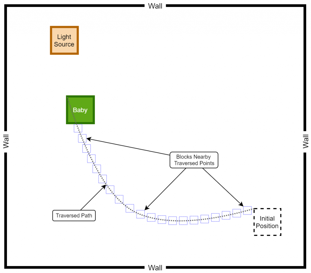

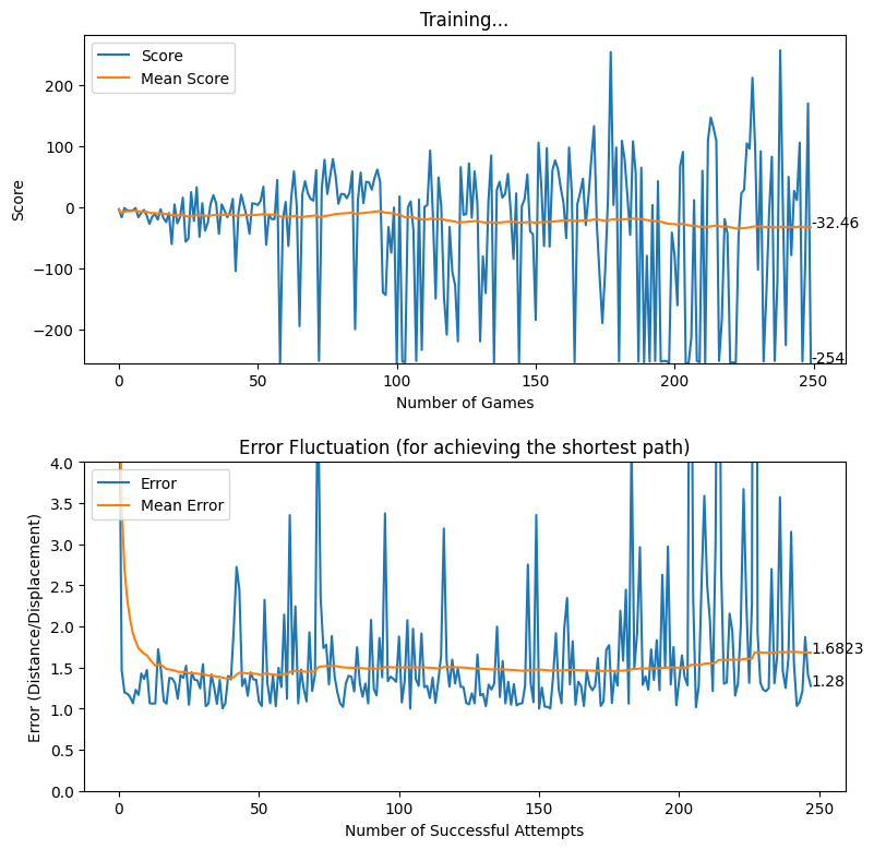
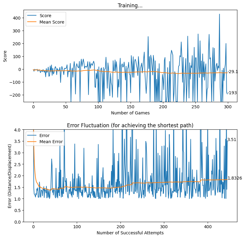
Rewarding based on Displacement Trail

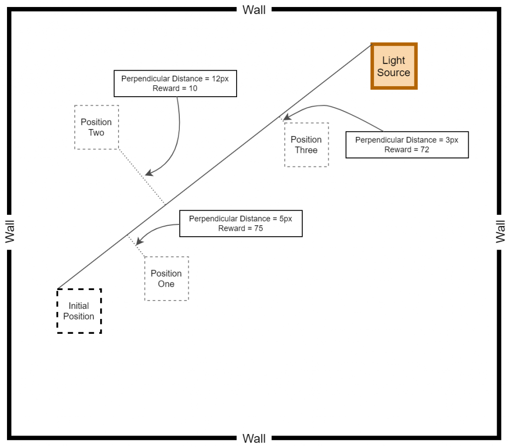
After many training sessions, we realized that the baby can actually self learn even with the availability of a much wider action space. However, so far, we have utilized the base rewarding mechanism explained here [hyperlink to appear here]. Additionally, we have introduced a negative rewarding mechanism for discouraging sub-optimal actions as explained in the previous section. Nonetheless, with the intention of improving the quality of actions made by the baby, we experimented with a new rewarding system where the baby is rewarded more for staying close to the displacement line. The thought process behind the implementation of this rewarding mechanism was that we wanted to encourage the baby to follow the shortest possible path while achieving the quest of reaching the destination.

reward = 0
game_over = False
current_position_x = baby.x
current_position_y = baby.y

if (baby collides with a wall) or (score < NEGATIVE_SCORE_THRESHOLD):
    game_over = True
    reward = -100

# If the baby is moving away, penalize by rewarding negatively.
if (baby moves away from the light source):
    reward = -20

# The baby must be rewarded for attempting to get close to the target.
if (baby gets close to the light source):
    # Calculate the perpendicular_distance between baby and the displacement line (between initial position and destination)
    reward = 75 - perpendicular_distance
    if reward >= 70:
      reward = reward
    else:
      reward = 10
          
# Discouraging sub-optimal actions
for traversed_point in traversed_points:
  if ((current_position_x < traversed_point.x + 1 ) and (current_position_x > traversed_point - 1)) and ((current_position_y < traversed_point.y + 1) and (current_position_y > traversed_point.y - 1)):
    reward = -50
    
# If the baby reaches the target, baby must be rewarded accordingly.
if (baby reaches light source):
    reward = 100

As explained above, the baby is heavily rewarded if the baby manages to stay within a perpendicular distance of 5 pixels on either side of the displacement line. In other cases, although the reward is positive, a relatively less reward is awarded for attempting to get close to the target. The following diagram provides a better understanding of how the displacement based rewarding mechanism is implemented.

After applying the aforementioned rewarding system, we observed that the baby attempts to move closer to the displacement line while reaching the target. We further observed that the as baby learns, the obstacles (walls) are avoided to the best effect, thus the game over states occur rarely.

Rewarding based on Optimum Future Moves (two levels)

In the previous section, we experimented with a reward mechanism that makes the baby focus on staying closer to the displacement line. Since we were able to get excellent results from the displacement-based reward system, it was decided to experiment with another approach where the baby is rewarded for taking optimum actions by searching through the future optimal action spaces. In this case, we started off by considering the action spaces only up to two levels because this is more of a brute-force approach where we check each and every possibility before making a move. In the long run, this kind of an approach can be infeasible due to the amount of processing power it needs to train the agent.

In this approach, as explained previously, the quality of potential future moves up to two levels are explored and the baby is rewarded heavily if the action taken by the neural network is a good move. Thus, the reward for each move depends on the optimality of the future moves.

Note: The following logic has been implemented using two different for-loops. However, this code can be optimized by using a recursive function.

def get_move_based_reward(self, action):
    # Maintaining a dictionary to store the distances between potential future moves, and the destination
    self.moves = defaultdict(dict)
    
    # Current moving angle is the last angle taken by the baby
    current_angle = self.angle_prev
    
    # Getting the current position of the baby
    head_position = self.head
    
    # Iterating through first level of future moves
    for angle in range(90,-100,-10):
    
        # Setting the future angle
        first_level_angle = current_angle
        first_level_angle += math.radians(angle)
        
        # Imaginarily placing the baby on the possile move of the first level 
        x = head_position.x + JUMP_DISPLACEMENT*math.cos(first_level_angle)
        y = head_position.y - JUMP_DISPLACEMENT*math.sin(first_level_angle)
        first_level_head_position = Point(x, y)
        
        # Iterating through the second level of future moves
        for second_angle in range(90, -100, -10):
        
            # Setting up the second level future angle
            second_level_angle = first_level_angle
            second_level_angle += math.radians(second_angle)
            
            # Imaginarily placing the baby on the possile move of the second level 
            second_x = first_level_head_position.x + JUMP_DISPLACEMENT*math.cos(second_level_angle)
            second_y = first_level_head_position.y - JUMP_DISPLACEMENT*math.sin(second_level_angle)
            second_level_head_position = Point(second_x, second_y)
            
            # Getting the distance between the destination and the position of the terminal level of tree
            distance_to_target = math.hypot(second_level_head_position .x - self.target.x, second_level_head_position.y - self.target.y)
            
            # Updating the dictionary
            if self.moves.get(str(angle)) is None:
                self.moves[str(angle)] = distance_to_target
            else:
                if self.moves[str(angle)] > distance_to_target:
                    self.moves[str(angle)] = distance_to_target

    # Sorting the dictionary of moves
    self.moves = dict(sorted(self.moves.items(), key = lambda item: item[1]))
    
    # Action <=> Angle Mapping
    # With this mapping, we get the angle suggested by the neural network as the next move.
    # As such, action_angle is the angle suggested by the neural network.
    action_index = action.index(1)
    action_angle = None
    angle_iterator = 0
    for angle in range(90, -100, -10):
        if angle_iterator == action_index:
            action_angle = angle
            break
        angle_iterator += 1

    # Calculating the distance between previous (last) actual position of baby and the destination
    # The calculated distance is then compared with the distances of potential future moves, and 
    # we get rid of potential future moves that are getting away from the target.
    # This gives us a ranked list of "good" potential future moves.
    prev_distance = math.hypot(self.head_prev.x - self.target.x, self.head_prev.y - self.target.y)
    self.moves = dict((k, v) for k, v in self.moves.items() if v <= prev_distance)
    
    # Checking if the action_angle (angle or move suggested by the neural network) exists in the 
    # list of "good" moves. The baby is then rewarded based on the action.
    if str(action_angle) in self.moves:         
        rank = list(self.moves).index(str(action_angle))
        reward = (75/len(self.moves))*(len(self.moves) - rank)
    else:
        reward = 0
    return int(reward)

While the above reward function works as expected, we later realized that the the final reward calculation retains a sense of biasness if the the number of “good” moves is less. Therefore, in the next iteration of our development, we introduced a slight change as follows.

   # Checking if the action_angle (angle or move suggested by the neural network) exists in the 
    # list of "good" moves. The baby is then rewarded based on the action.
    if str(action_angle) in self.moves:         
        rank = list(self.moves).index(str(action_angle))
        if rank < 5:
          reward = 75 - rank*5
        else:
          reward = 10
    else:
        reward = 0

Working with a grid of obstacles

In the section "Working with Obstacles", we discussed about the inclusion obstacles to make it difficult for the baby to learn the end goals. Nevertheless, it did not end up becoming a hurdle for the baby as the baby comfortably managed to avoid the obstacles. However, we utilized only two obstacles at a time for the sake of simplicity. As per our next set of experiments, it was decided to include a grid of obstacles to make it look like a maze, as shown in the following diagram.

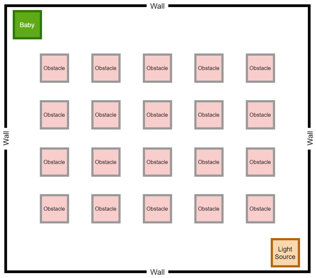
Surprisingly (or not surprisingly), after some hours of training, the baby managed to find his/her way towards the destination while avoiding the grid of obstacles. As we had experimented with two types of rewarding mechanisms (displacement-based and optimum future moves-based), the game was trained using both rewarding systems separately, and we certainly received excellent results in both types of rewarding systems.

Optimum Future Moves based Reward

In this case, the optimum future moves were implemented, but compared to the explanation given previously, this time around, we went ahead with three levels of depth search instead of two levels. The results are impressive as shown in the following video clips.

Displacement based Reward

In a similar manner with the grid of obstacles, the game was trained with the displacement-based reward system and the results are illustrated below.