Fidenz at WebSummit 2025

Your Partner in Scalable SaaS Product Development
At Fidenz Technologies, we specialize in building robust, scalable SaaS platforms for startups and enterprises. With over a decade of experience serving clients across the Nordics, North America, and APAC regions, we bring deep technical expertise and a strong product mindset to the table.
This year again, we are coming back to join Websummit2025 to connect, collaborate, and co-create with like-minded innovators in the SaaS community.
Why Work With Us?
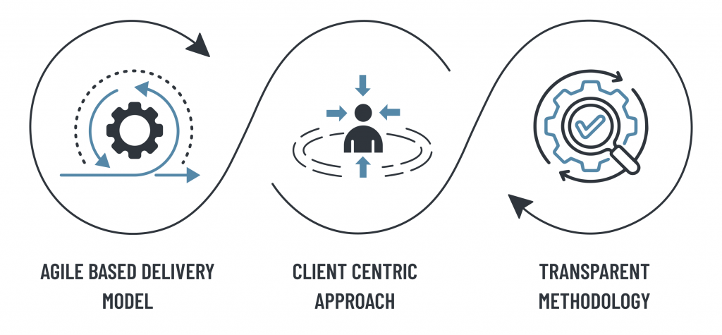
✅ 15+ Years Serving the Nordics
✅ Product-Driven Engineering – We don’t just build software, we build businesses. Our team thinks long-term and aligns with your vision.
✅ Agile Delivery, Zero-Dependency Model – Flexible, client-centric processes that ensure reliable delivery with speed and transparency.
✅ SaaS-Specific Expertise – From MVPs to enterprise-grade platforms.
What We Offer
- Full-cycle SaaS Product Development
- MVP to Enterprise-Grade Platform Builds
- Cloud Infrastructure (AWS, GCP, Azure)
- DevOps, CI/CD, Docker, Kubernetes
- Third-Party Integrations & API Management
- Data Architecture, Analytics, Dashboards
- UX/UI, QA & Ongoing Support
Build With Skilled Remote Engineers
Whether you need to scale up fast, augment your team, or outsource an entire project, our vetted remote engineers deliver with agility, reliability, and zero long-term dependencies.
✅ On-demand team scaling
✅ Clear, documented processes
✅ Seamless collaboration
✅ Time-zone alignment for global teams
Our Approach
We Are Global

With an office in Oslo and delivery teams in Colombo, Sri Lanka, we’ve built strong and long-term partnerships across the Nordics.
We grow with our clients; when they succeed, we move forward together. That’s why we invest in building relationships.
Few Nordic Clients
Tools We Use

Let’s Meet at WebSummit2025
We'd love to hear about your SaaS journey and see how we can contribute to your growth. Whether you’re looking to scale, modernize, or launch something new, let’s talk!
📍 Location: MEO Arena | Lisbon
📅 Date: November 10 - 13
![]() Chat on the WebSummit 2025 App: https://attend.websummit.com/lis25
Chat on the WebSummit 2025 App: https://attend.websummit.com/lis25
Get In Touch
Book our calendar ![]() http://calendly.com/chim/ or,
http://calendly.com/chim/ or,
Fill out the form below ![]()
https://forms.gle/hc8f7DoGYunGpAuDA
And let’s schedule a quick 1:1 chat during the event or after.
Connect with us!
![]() +47 939 37 942
+47 939 37 942
Fidenz at SaaSiest 2025

Your Partner in Scalable SaaS Product Development
At Fidenz Technologies, we specialize in building robust, scalable SaaS platforms for startups and enterprises. With over a decade of experience serving clients across the Nordics, North America, and APAC regions, we bring deep technical expertise and a strong product mindset to the table.
This year, we are excited to join SaaSiest 2025 to connect, collaborate, and co-create with like-minded innovators in the SaaS community.
Why Work With Us?
✅ 10+ Years Serving the Nordics
✅ Product-Driven Engineering – We don’t just build software, we build businesses. Our team thinks long-term and aligns with your vision.
✅ Agile Delivery, Zero-Dependency Model – Flexible, client-centric processes that ensure reliable delivery with speed and transparency.
✅ SaaS-Specific Expertise – From MVPs to enterprise-grade platforms.
What We Offer
- Full-cycle SaaS Product Development
- MVP to Enterprise-Grade Platform Builds
- Cloud Infrastructure (AWS, GCP, Azure)
- DevOps, CI/CD, Docker, Kubernetes
- Third-Party Integrations & API Management
- Data Architecture, Analytics, Dashboards
- UX/UI, QA & Ongoing Support
Built with Skilled Remote Engineers
Whether you need to scale up fast, augment your team, or outsource an entire project, our vetted remote engineers deliver with agility, reliability, and zero long-term dependencies.
✅ On-demand team scaling
✅ Clear, documented processes
✅ Seamless collaboration
✅ Time-zone alignment for global teams
Our Approach
We Are Global
With an office in Oslo and delivery teams in Colombo, Sri Lanka, we’ve built strong and long-term partnerships across the Nordics.
We grow with our clients; when they succeed, we move forward together. That’s why we invest in building relationships.
Few Nordic Clients
Tools We Use
Let’s Meet at SaaSiest 2025
We'd love to hear about your SaaS journey and see how we can contribute to your growth. Whether you’re looking to scale, modernize, or launch something new, let’s talk!
📍 Location: Malmö, Sweden
📅 Date: May 6–7, 2025
![]() Chat on the Saasiest App: The world's leading event & networking platform
Chat on the Saasiest App: The world's leading event & networking platform
Get In Touch
Book our calendar ![]() http://calendly.com/chim/ or,
http://calendly.com/chim/ or,
Fill out the form below ![]()
And let’s schedule a quick 1:1 chat during the event or after.
Connect with us!
![]() +47 939 37 942
+47 939 37 942
Fidenz in Oulu

Skilled Remote Engineers to expand your delivery capacity
Hire an engineering team, add engineers to your existing team, or get a project done in a Cost-Effective way
Fidenz Technologies is a trusted software development partner serving the Nordics for over a decade. Bootstrapped by engineers, we bring together a team of 40+ professionals offering end-to-end services from system architecture, design, development, testing, cloud infrastructure, deployment, UI/UX, quality assurance, documentation and support.
Services We Offer
- Web and Mobile-based SaaS platform development
- Hardware integrations and IoT systems (Bluetooth, Device Drivers, RS232)
- Cloud infrastructure management (AWS, GCP, Azure), including Kubernetes, and Docker
- Process automation for industrial and connected environments
- Data and Event management using Kafka, MQTT, InfluxDB, Prometheus, and Elastic Search
- Data analytics and visualization
Our Approach
Countries We Serve

With an office in Oslo and delivery teams in Colombo, Sri Lanka, we’ve built strong and long-term partnerships across the Nordics.
We grow with our clients; when they succeed, we move forward together. That’s why we invest in building relationships.
Few Nordic Clients
Tools We Use
We are coming to Oulu!
– Come and meet us –

If you would like to connect with us one-to-one before or after the event, feel free to set up a meeting http://calendly.com/chim/
Connect with us!
+47 939 37 942
KESA – Event Sourcing
KESA - Event Sourcing Illustrated: A Jigsaw Puzzle Game Perspective
In the dynamic world of software development, managing and maintaining the state of an application poses significant challenges. Event sourcing, an innovative architectural pattern, steps in to revolutionize this process, which offers a robust foundation for understanding not only where the system stands, but also how it got there, significantly enhancing both transparency and traceability.
What is Event Sourcing?
Event sourcing is an architectural pattern that captures changes to an entity's state through a chronological series of events. This approach diverges from traditional methodologies that emphasize storing the current state, by instead focusing on the sequence of events that lead to that state.
Event Sourcing utilizes concepts such as events, event streams, event stores, and event handlers to manage and process these changes. Further, it offers benefits such as immutable event logs, auditability, event replay for state reconstruction, consistency, improved scalability, fault tolerance, and support for event-driven architectures.
Jigsaw Puzzle Game Project Overview
To illustrate the practical application of event sourcing, we present a simple, engaging example: a digital jigsaw puzzle game. This single-player game is developed to highlight the principles and advantages of event sourcing and event-driven architectures, where a player interacts with a web interface to assemble a jigsaw puzzle.
Play the game here: Fidenz Kesa
Find instructions on how to play here
Find the full project explainer video here: https://youtu.be/4O9VukIrtCI
Implementing Event Sourcing in Jigsaw Puzzle Game
The table below demonstrates the implementation of event sourcing features within the Jigsaw Puzzle Game application, which has been intentionally over-engineered to effectively illustrate event sourcing capabilities using a jigsaw puzzle game as an example.
| Event Sourcing Feature | Application Implementation | Benefits in the Game Context |
|---|---|---|
| Entity | The "JigsawPuzzleGame" entity is designed to represent the current state of a gaming session. | Encapsulates the game logic and helps validating events for an ongoing gaming session |
| Event | Each game action triggering an event sent from the front-end to the back-end such as: Game Started Event, Piece Added Event, Piece Removed Event. | Facilitates real-time game interactions and state management |
| Event Stream | A gaming session begins with a Start Game Event, marking the commencement of an event stream. Subsequent events, including Piece Added Events and Piece Removed Events, will be sequentially numbered in chronological order. | Ensures ordered, reliable processing of game actions |
| Event Handlers | Event handlers are designed to react to various events, taking actions such as processing data and updating “JigsawPuzzleGame” entity. | Enables dynamic game state management based on player actions |
| Event Store | Events are stored in the event store and can be retrieved as needed. Once saved, these events are immutable. Each event record includes essential information such as the unique game session ID, event type, event stream ID, and event data, among other details. | Provides durability and historical tracking of game actions |
| Immutable Event Log | Event Store implementation provide chronologically ordered immutable events of a gaming session | Accurate tracking of puzzle progress |
| Event Replay | A Player can use the Event List to go back in time to a specific point in the game. This can be done by selecting an event from the event list. The system then reverse all subsequent events by applying their opposite, thus restoring the puzzle to the desired state |
Ability to revert puzzle state and understand puzzle assembly |
| Consistency and Eventual Consistency | Storing events in chronological order with event stream ID and event type | Distinguishes between the various events that occur within a gaming session. |
Conclusion
The jigsaw puzzle game serves as a practical and engaging example to illustrate the principles of event sourcing. By understanding how each action in the game translates into an event and contributes to the puzzle's state, we can appreciate the power and utility of event sourcing in software development. As technology evolves, it's exciting to ponder how event sourcing will shape the future of data management and application design.
Would you like to learn more? Contact Us!
If you have any additional questions about this or would like a word with our creators? Feel free to reach out to us.
📆 Talk to Us: Contact us - Fidenz Technologies
Keep an eye out for our upcoming content from Fidenz Technologies, as we embark on a journey through the intricate realms of technology.
Happy Exploring!
Instructions and How to play this game
- Watch the video below for instructions on how to play the game.
- Interact with a dual-panel interface: left panel for puzzle assembly, right panel for displaying available jigsaw pieces.
- First, choose a puzzle size from three game size options: 4x4, 5x5 (default), or 6x6.
- Start the game using start button
- Upon start four puzzle pieces will be available in the piece viewer for selection.
- Add pieces by dragging them from the piece viewer to the grid.
- Remove pieces by clicking on a piece in the grid and confirming the subsequent pop-up.
- Removed pieces won't be added back to the piece viewer but will be available for future selection.
- Use the “Re-shuffle” button to refresh the piece selection with a new set of random pieces, useful when the piece viewer is empty.
- Reset the game at any time using the “Reset” button.
- Event List Panel
- To view the events occurred while playing the game
- To Revert puzzle to a previous state by selecting an event in the event list and confirming the prompted pop-up.
The game concludes when the puzzle is fully assembled, with completion time affecting the player's score.
Why Kubernetes On-Prem and a Glimpse into Our Setup
Introduction
Deploying a Kubernetes on-prem cluster may pose challenges, but it grants complete control over hardware, allowing customization of infrastructure to specific needs. Data is stored securely within our organization's premises, eliminating recurring costs for the same resources. Additionally, the setup allows for performance optimization and avoids network overhead.
let's see why we would need a Kubernetes on prem cluster.
Why Kubernetes On-Prem?
Embarking on the deployment of a Kubernetes cluster on-premises is undeniably accompanied by inherent challenges; however, there exist compelling scenarios that necessitate this strategic decision. The stringent demands of regulatory compliance, coupled with heightened security considerations, often drive organizations towards on-premises deployment. Furthermore, the seamless integration with pre-existing infrastructure and the pursuit of optimized performance, especially in scenarios requiring low-latency workloads, reinforce the appeal of on-premises Kubernetes deployment. In the intricate landscape of modern IT, these considerations collectively underscore the relevance of on-premises solutions despite their inherent complexities.
How we deployed our own Kubernetes on-Prem cluster
When considering the deployment of a Kubernetes on-premises cluster, it's essential to take into account factors such as the storage provisioner, load balancing, cluster autoscaling, and high availability. We opted for a canonical stack to facilitate the deployment of our on-premises cluster, aiming to achieve automated cluster deployment and configure high availability seamlessly.
We leveraged MAAS (Metal as a Service) for infrastructure provisioning. MAAS is a robust tool that streamlines the deployment of physical servers, allowing for efficient management and provisioning in a data center or on-premises environment.
To orchestrate the cluster deployment, we employed Juju. Juju is a powerful application modeling tool that simplifies the management and scaling of complex software infrastructure. It facilitates the seamless deployment and integration of applications across various cloud and on-premises environments.
Now, let's delve into the steps and measures we undertook to successfully deploy our own Kubernetes on-premises cluster
Features provided by our on-premise Kubernetes cluster
- Persistent Storage
- We chose Ceph as our storage provisioner, leveraging Juju for both the deployment and configuration of the Ceph cluster. With features like storage pooling and replication, Ceph ensures a highly available storage provisioner, meeting our requirements for resilience and redundancy in the storage infrastructure.
- High Availability
- With Juju, we could deploy multiple control nodes, ensuring easy availability, and set up multiple etcd and Ceph servers for enhanced resilience and availability. This approach enhances the reliability of our infrastructure by distributing critical components across redundant nodes, minimizing the risk of single points of failure.
- Cluster Autoscaling
- Utilizing the Charmed Kubernetes Autoscaler, we've automated node autoscaling within our Kubernetes cluster, dynamically adding or removing worker nodes as needed. This not only ensures optimal resource utilization but also contributes to cost efficiency by automatically adjusting the cluster size based on workload demands. The autoscaler is a valuable tool for maintaining an agile and resource-efficient on-premises Kubernetes environment.
- Load Balancing
- With the integration of MetalLB as our load balancer, we enhance the scalability and distribution of network traffic within the cluster. MetalLB is a versatile load balancing solution designed for bare-metal Kubernetes deployments. It dynamically assigns external IP addresses to services, allowing for efficient load balancing and seamless traffic management across the Kubernetes nodes in our on-premises cluster.
Feel free to refer to our second article for a more in-depth exploration of why we opt for Kubernetes on-premises and a detailed comparison highlighting the distinctions between on-premises and cloud deployments.
Now, please head down to our video to delve a bit deeper into these topics and take a closer look at our deployed Kubernetes on-premises cluster.
📽️ Watch Video: Why Kubernetes On-Prem and a Glimpse into Our Setup
Would you like to learn more? Contact Us!
If you have any additional questions about this or require a similar service, feel free to reach out to us. We're here to assist you and explore how we can meet your specific needs.
📆 Talk to Us: Talk to Creators
Keep an eye out for our upcoming content from Fidenz Technologies, as we embark on a journey through the intricate realms of technology. Join us for in-depth explorations, insightful discussions, and a continuous stream of technological adventures that promise to expand your knowledge and keep you informed about the latest trends and developments in the ever-evolving tech landscape.
Until then, happy exploring!
Fidenz’s Software Quality Assurance Process
Overview
Reliability of a software product plays a crucial role in determining the success of a product and maximizing the return on investment. And achieving the highest possible reliability is a process that involves carefully balancing various factors, mainly time and cost. In this article, we will explore the QA process at Fidenz and how it is tailored to achieve optimal reliability while balancing the cost and time.
Software Product Reliability
What is our perspective on software product reliability?
In our perspective, software product reliability is the software system's ability to consistently function without failure over a specific period. It emphasizes stability, consistent performance, and minimal downtime.. Achieving software product reliability involves rigorous testing, quality assurance, and proactive issue resolution during development. Also involves carefully balancing various factors, mainly time and cost.
Cost and Time Dependency
The relationship between these two factors often involves trade-offs. For example, enhancing reliability may require additional resources and time to conduct comprehensive testing and quality assurance procedures. Similarly, reducing costs might lead to compromises in reliability or extended project timelines. Additionally, adhering to strict time constraints might result in increased costs or reduced reliability.
QA process at Fidenz is designed to achieve optimal reliability while balancing the cost and time.
Quality Assurance Process at Fidenz
We employ various testing methodologies and techniques at Fidenz. Let's take a closer look at three important types of test automation.
- Unit Testing
- Test automation with Cypress
- Stress Testing
We also recognize that every software system is unique, and as such, we prioritize the development of custom testing strategies tailored to the specific requirements of each project. This approach not only reduces costs, But also, ensures that essential testing aspects are covered for every project.
What is QA Automation?
QA automation, or Software quality assurance automation, refers to the process of using specialized software tools and frameworks to automate the execution of tests on software applications. This approach aims to enhance the efficiency and accuracy of software testing by reducing manual intervention and human error.
QA Automation Benefits
- Time
- Faster Testing: Automated tests can execute much faster than manual tests, enabling rapid validation of software changes and shorter development cycles.
- Cost
- Cost Savings: While there is an initial investment in creating and maintaining automated test suites, it leads to long-term cost savings by reducing the need for manual testing resources and allows shipping changes and enhancements to production in minimum time
- Reliability
- Improved Test Coverage and Code Quality: Automation allows for comprehensive testing of various scenarios, ensuring that critical aspects of the software are thoroughly examined.
- Early Defect Detection: Automation detects defects as soon as new code is integrated, allowing for immediate feedback to developers, which helps in addressing issues promptly and reducing development costs.
Continuous Integration
We utilize CI/CD services such as Bitbucket Pipelines and GitHub Actions to streamline the automated test script execution. This approach guarantees that the code undergoes automated testing before advancing to the QA phase and deployment.
Upon each repository update, the system runs unit tests and test automation scripts. Timely test reports are sent via email to pertinent project stakeholders, facilitating prompt actions as required.
Would you like to learn more? Contact Us!
For more information and updates on QA automation process at Fidenz, stay tuned. Follow us for the latest updates!
📽️ Watch Video: Software Quality Assurance Process at Fidenz
📆 Talk to Us: Fidenz Technologies
KEDAS: Sync relational and non-relational databases using Kafka
Background
In the era of digitalization, the landscape of data has evolved dramatically. Initially used for monitoring and analysis, data quickly became a vital asset for real-time decision-making. As data volumes soared, the value of static information dwindled, while the significance of continuous data streams skyrocketed. Within this dynamic context, Kafka emerged as a pivotal tool for data management.
What is Kafka?
Kafka lies at the heart of this data revolution as an event streaming platform. It excels at capturing data from diverse sources, seamlessly processing, storing, and delivering it to those who seek actionable insights. While Kafka shares similarities with traditional pub-sub message queues like RabbitMQ, it sets itself apart in several critical ways:
- Operates as a modern distributed system
- Offers robust data storage capabilities
- Processes data streams, creating new events beyond traditional message brokering
Purpose of this Project
Recognizing Kafka's versatility and surging popularity, we embarked on a journey to harness its capabilities for delivering superior solutions to our clients.
Our mission? To dive deep into this technology and build an innovative solution leveraging Kafka’s capability.
Project Overview
KEDAS is a data synchronization application designed to work seamlessly across various database servers, including MS SQL, MySQL, PostgreSQL, and more. In an effort to enhance versatility and complexity, we extended its capabilities to facilitate synchronization between both relational and non-relational databases. Unlike most data synchronization tools available, our solution allows changes made in one data source to be seamlessly synchronized with multiple data sources through minimum configurations.
This project stands as a testament to our commitment to embracing innovative technologies like Kafka to offer cutting-edge solutions to our clients. As data continues to be a driving force in the digital landscape, Kafka remains at the forefront of efficient and real-time data management, enabling us to deliver exceptional results.
Outcomes
We have developed a Kafka processor and a set of Kafka connectors to enable data synchronization between different data sources. To make the system testable, we have developed a simple web application that interacts with two independent databases which are synchronized using our KEDAS.
Kafka Demo App
Check out the video below to get a quick overview of how everything works together and if you like to try how this works, try it yourself with our demo application.
Demo Video: Kedas Demo
Try it yourself: Kedas Dashboard
Want to know more about Kafka based solutions? Talk to Creators
For more information and updates on Kafka-driven projects by Fidenz, stay tuned. Follow us for the latest updates!
Case Study – Self Navigator
Introduction
If you are capable of reading this piece of text, it is certain that you have passed your infancy. As someone who has come a long way from infancy, did you ever think of how you LEARNED to stand-up, walk, and basically avoid the dangers? If you start to deeply analyze the whole phenomenon behind your journey, you will realize that you LEARNED FROM EXPERIENCE with every passing moment of your life. Isn’t it beautiful how the experience allowed you to be yourself, and explore the world to be where you are now?
Combined with the experience and the inputs acquired by the five senses, the human evolves through a journey of lifetime, while facing a vast array of successes, sorrows, challenges, and emotions. For instance, during your lifelong learning experience, if you are REWARDED for an action that you performed with goodwill, more often than not, you will be inclined to perform the same action at least few more times if it is guaranteed that you are rewarded for your actions. On the other hand, it is almost certain that you will end up restricting yourself from doing non-acceptable actions that heavily PENALIZE you. Irrespective of the task/action, this is a process that has inherently assisted us in making informed decisions based on the past experiences. Here, why do you think that we are we interested in the basic decision making process employed by the human? In this article, we will look into the possibilities of teaching the machines to mimic the experience-based human reasoning process, and we will show you a demonstration of how it is achieved in a methodical approach.
Analogy
Before diving into the technical aspects of the theory behind this approach, let us try to map our problem to a fundamental problem. Imagine that you are a baby who is stuck in a dark room, and you have no clue whatsoever on what you should do next. Since you are a baby, you do not have any idea about the surroundings, and unfortunately, you do not have anyone to ask for help. However, you have the option of taking baby steps forward or right or backward or left. At the same time, suppose that you have a stock of chocolate (100 g) in your hand, and you really love them. Well, who doesn’t? Nonetheless, you can see light waves coming towards you from the other side of the room (possibly a way to get out of darkness). Gradually, you take random steps, and to your surprise, you realize that the stock of your chocolate changes depending on the actions you take, as follows.
- Whenever you touch a wall of the dark room, you lose 20 g of chocolate.
- For each baby step taken by you, if it gets you closer to the light waves, your chocolate stock gets increased by 2 g. If you move away from the light waves, you are penalized by taking 10 g of chocolate away from you.
- If you somehow manage to reach the source of light waves, you are given 100 g of chocolate.
Since the baby loves chocolates, the baby begins realizing the pattern that benefits him/her more and the baby eventually reaches the source of light waves. This is an interesting analogy to imply how the baby’s brain picks the more rewarding patterns while avoiding patterns that negatively impact the baby.
While it is tempting to understand how a human picks such patterns, what would you say if we can convince you that the computer is also capable of mimicking the human behaviour in terms of self learning and pattern recognition? Reinforcement Learning is an interesting research area that allows us to achieve the task of making computers recognize such patterns, and with this article, it is expected to bring you an understanding of how it can be achieved.
Reinforcement Learning
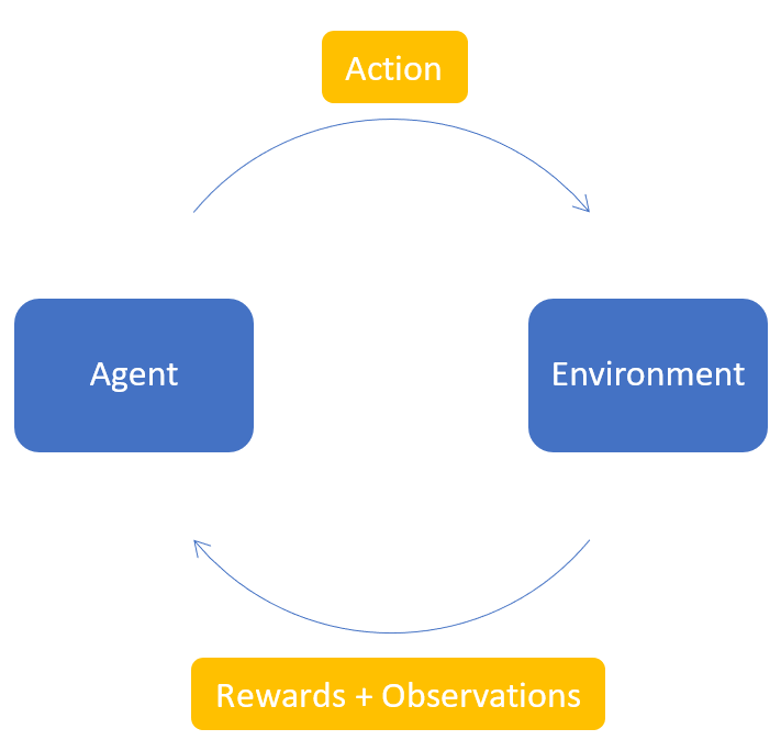
Reinforcement Learning (RL) focuses on teaching agents through trial and error. It learns by actively engaging with an environment. It consists of four fundamental concepts that make up as the building blocks of Reinforcement Learning.
- Agent: The entity (actor) that operates in the environment according to a policy
- Environment: The world in which the agent operates in
- Action: The possible action done by the agent
- Rewards: The points received by the agent upon performing an action, based on its actions on the environment.
- Observations: The observations available after performing the action
If we can consider and compare the analogy explained previously with the concepts of Reinforcement Learning, the following mapping can be illustrated.
| Agent | ↔︎ | Baby |
| Environment | ↔︎ | The Dark Room |
| Action | ↔︎ | Forwards, Right, Backwards, Left |
| Rewards | ↔︎ | Chocolates |
| Observations | ↔︎ | Baby realizing what happened after performing an action |
Reinforcement Learning behaves as the foundation for our goal, and the concepts of Q-Learning and Deep Q-Learning can be employed as aids to implement the solution. In the following sections, the concepts behind Q-Learning and Deep Q-Learning are briefly explained.
Q-Learning
As explained previously, the reward awarded for each action at each step is a known element within our framework. The agent is supposed to carry out a sequence of actions to maximize the total reward where the total reward can be termed as the Q-value. The Q-value can be obtained as follows.
Q(s,a) = r(s,a) + γ max Q (s',a)
In the formula, the Q value for performing the action a at state s is obtained by considering the existing reward [r(s,a)] and the highest possible Q-value obtainable from the state s' (next state). In this equation, γ (Gamma) is the discount factor which determines the contribution of the future rewards.
Since this acts as a recursive function, Q(s’,a) depends on Q(s”,a) and we essentially get a recursive function. As such, we initialize the model by initializing a Q value, and then let the agent choose a suitable action. The chosen action could be a predicted action or a random action if the agent is at the early stages of training. Based on the chosen action, the action is performed and its reward is measured before updating the Q value. This sequence of steps (except the initialization of Q value) is repeated during the training process.
Deep Q-Learning
The combination of Q-Learning and Deep Learning enables us to utilize Deep Q-Learning where we finally get a neural network for taking the optimum actions. While the usual Q-Learning can be used for simple tasks, it can be infeasible in occasions where we have a large number of states along with a big action space. This is where the concepts of neural networks become handy as it allows the agent to approximate the values of the Q-learning function. In this neural network, we utilize the Mean Squared Error as our loss function, which can be illustrated as follows.
loss = (Qnew - Q)^2 where the Q values can be obtained using the Bellman’s equation given above.
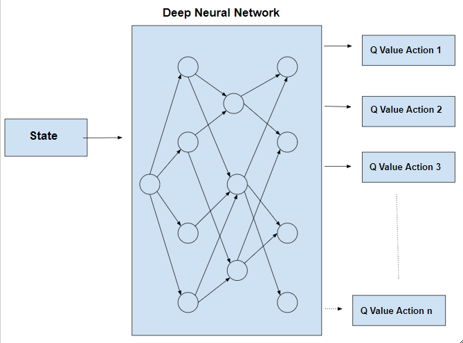
In the above neural network, we choose the action that corresponds to the maximum Q value among the n number of actions given as the output. More information regarding how these theorems are applied to our use case, are given in the subsequent sections.
Implementation of Analogy
For the sake of simplicity, we will create a simple 2D game that can represent the previously explained analogy where both the baby and the light wave sources are represented by squares (different colours). The game is encapsulated by four walls (borders of the 2D game), and the baby is rewarded or penalized based on the actions taken. On the other hand, if the baby somehow manages to reach the light source, the baby is heavily rewarded. The entire game is presented to the audience as if the audience is watching the game from an aerial view as it provides the best possible view to understand the course of actions.
In the meantime, we will also mention a score that the baby can accumulate over different episodes within the game. If the baby manages to reach the light source, the light source will be randomly placed somewhere else within the room, and the baby will have to go to the new position of the light source. The game scoring rules will be as follows.
- Baby can take the following actions where the baby will move by a unit distance on the given direction.
- Forward
- Backward
- Left
- Right
- Baby takes a step:
- If the step results in baby getting closer to the light source → +1 point
- If the step results in baby getting away from the light source → -5 points
- If baby reaches the light source → +50 points (light source will get placed at a different location after obtaining +50 points)
- If baby hits one of the walls → Game Over
Based on the defined game rules and the expected goal, it is expected to implement the game as shown in the following sketch.
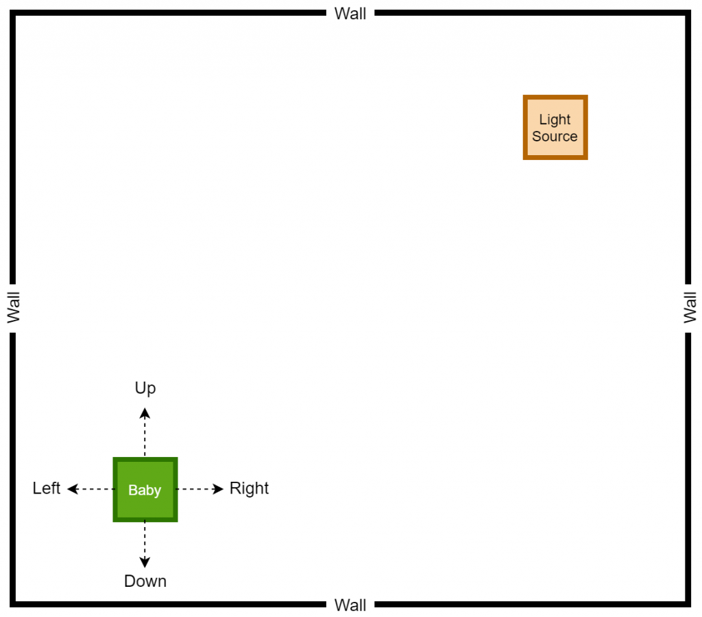
The Up, Right, Down, and Left arrows represent the actions that can be performed by the baby, and the corresponding directions are assigned by assuming that the game is controlled from an aerial position. As it stands, our goal is to teach the baby to take the correct actions to reach the light source, and it is performed by rewarding or penalizing the baby based on the actions taken by the baby himself/herself.
We will first attempt to create a game that can be played by a human where the keyboard controls can be used to control the actions taken by the baby. Afterwards, we will work on creating a computer agent along with a deep learning model that can effectively mimic the human behaviour to eventually automate the actions taken by the baby.
The Game
The game will be implemented by considering Python as the programming language, and we also employ the services of a Python 2D game library known as PyGame. As usually, it is required to utilize a Python environment for the purpose of creating this game, and we encourage you to install the PyGame library as a prerequisite.
Game (Played by a human)
Once the prerequisites are satisfied, we implemented the human-playable game where the code is self-explanatory with the given comments.
game.py
import pygame
import random
from enum import Enum
from collections import namedtuple
import math

pygame.init()

font = pygame.font.Font('arial.ttf', 25)

# Possible directions of the Baby
class Direction(Enum):
    RIGHT = 1
    LEFT = 2
    UP = 3
    DOWN = 4

Point = namedtuple('Point', 'x, y')

#RGB Colours
WHITE = (255, 255, 255)
BLACK = (0, 0, 0)
GREEN1 = (107,142,35)
GREEN2 = (173,255,47)

BLOCK_SIZE = 20
SPEED = 3
NEGATIVE_SCORE_THRESHOLD = 20

class Baby():

    def __init__(self, w = 640, h = 480):
        self.w = w
        self.h = h

        # Initialize the Display
        self.display = pygame.display.set_mode((self.w, self.h))
        pygame.display.set_caption('Path Finder')
        self.clock = pygame.time.Clock()

        # Initialize the game state and place the target
        self.direction = Direction.LEFT
        self.head = Point(self.w/2, self.h/2)
        self.head_prev = Point(self.w/2, self.h/2)

        self.score = 0
        self.target = None

        self._place_target()

    def _place_target(self):
        # Place the target inside the window
        x = random.randint(0, (self.w - BLOCK_SIZE) // BLOCK_SIZE) * BLOCK_SIZE
        y = random.randint(0, (self.h - BLOCK_SIZE) // BLOCK_SIZE) * BLOCK_SIZE
        self.target = Point(x, y)

        # To ensure that the target does not get placed on the Baby
        if self.target == self.head:
            self._place_target()

    def play_step(self):

        # Collect user input
        for event in pygame.event.get():
            if event.type == pygame.QUIT:
                pygame.quit()
                quit()

            if event.type == pygame.KEYDOWN:
                if event.key == pygame.K_LEFT:
                    self.direction = Direction.LEFT
                elif event.key == pygame.K_RIGHT:
                    self.direction = Direction.RIGHT
                elif event.key == pygame.K_UP:
                    self.direction = Direction.UP
                elif event.key == pygame.K_DOWN:
                    self.direction = Direction.DOWN

        # Move the Baby
        self._move(self.direction)  # Update the head

        # Check if the game is over
        game_over = False
        if self._is_collision() or self.score < -NEGATIVE_SCORE_THRESHOLD:
            game_over = True
            return game_over, self.score

        # If the Baby is moving away, penalize
        if self._is_moving_away():
            self.score -= 5

        # If the Baby is getting close, reward
        if self._is_moving_close():
            self.score += 1

        # Place new target or move the Baby
        if self.head == self.target:
            self.score += 10
            self._place_target()

        # Update UI and clock
        self._update_ui()
        self.clock.tick(SPEED)

        # Return if the game is over and score
        return game_over, self.score

    def _is_collision(self):
        # Does it hit the boundary?
        if (self.head.x > self.w - BLOCK_SIZE) or (self.head.x < 0) or (self.head.y > self.h - BLOCK_SIZE) or (self.head.y < 0):
            return True
        return False

    def _is_moving_away(self):
        prev_distance = math.hypot(self.head_prev.x - self.target.x, self.head_prev.y - self.target.y)
        current_distance = math.hypot(self.head.x - self.target.x, self.head.y - self.target.y)
        if current_distance > prev_distance:
            return True
        return False

    def _is_moving_close(self):
        prev_distance = math.hypot(self.head_prev.x - self.target.x, self.head_prev.y - self.target.y)
        current_distance = math.hypot(self.head.x - self.target.x, self.head.y - self.target.y)
        if current_distance > prev_distance:
            return False
        return True

    def _move(self, direction):
        x = self.head.x
        y = self.head.y
        self.head_prev = Point(x, y)

        if direction == Direction.RIGHT:
            x += BLOCK_SIZE
        elif direction == Direction.LEFT:
            x -= BLOCK_SIZE
        elif direction == Direction.DOWN:
            y += BLOCK_SIZE
        elif direction == Direction.UP:
            y -= BLOCK_SIZE

        self.head = Point(x, y)

    def _update_ui(self):
        self.display.fill(BLACK)

        # Drawing the Baby
        pygame.draw.rect(self.display, GREEN1, pygame.Rect(self.head.x, self.head.y, BLOCK_SIZE, BLOCK_SIZE))
        pygame.draw.rect(self.display, GREEN2, pygame.Rect(self.head.x + 4, self.head.y + 4, 12, 12))

        # Drawing the Target
        pygame.draw.rect(self.display, WHITE, pygame.Rect(self.target.x, self.target.y, BLOCK_SIZE, BLOCK_SIZE))

        text = font.render("Score: " + str(self.score), True, WHITE)
        self.display.blit(text, [0, 0])
        pygame.display.flip()

if __name__ == '__main__':
    game = Baby()

    # Game Loop
    while True:
        game_over, score = game.play_step()

        # Break if the game is over
        if game_over == True:
            break

    print('Final Score: ', score)

    pygame.quit()
Next, we create an agent that can effectively make the computer learn by playing the game. However, it is also important to initialize a deep learning model that gets trained based on the actions performed by the agent.
Reward Function
The reward function plays a critical role in making the computer learn all the “Good” and “Bad” actions that it can learn. For instance, our goal is to positively reward for all the good actions and to negatively reward for bad actions. At the same time, we have attempted to quantify the “goodness” and “badness”, as it gives the computer a degree of freedom in learning.
As shown in the following pseudocode, the baby is rewarded negatively for each move that results in a collision with one of the four walls. Similarly, if the baby is trying to move away from the light source, for each move that results in an away movement, the baby is rewarded negatively. It should be noted that the collision avoidance has a higher priority, and as a result, the negative reward for collision avoidance has a higher magnitude compared to away movement. In a similar manner, the baby is positively rewarded for getting close to the light source, and for reaching the target.
reward = 0
game_over = False

if (baby collides with a wall):
    game_over = True
    reward = -10

# If the baby is moving away, penalize by rewarding negatively.
if (baby moves away from the light source):
    reward = -5

# The baby must be rewarded for attempting to get close to the target.
if (baby gets close to the light source):
    reward = 5

# If the baby reaches the target, baby must be rewarded accordingly.
if (baby reaches light source):
    reward += 10
In the following code blocks, the behaviour of both the agent and the model are demonstrated.
Agent
The agent takes care of the task of training the baby to identify the patterns and eventually learn what affects the baby most. The agent utilizes both the game environment and the created model to handle and coordinate the sequences of actions within the game. As shown in the code itself, the agent creates two objects, one from the game environment and the other one from the model. Further, some of the model hyperparameters are also set by the agent, and such hyperparameters are provides as inputs during the model creation time.
agent.py
import torch
import random
import numpy as np
from collections import deque
from game import BabyRL, Direction, Point
from model import Linear_QNet, QTrainer
from helper import plot

MAX_MEMORY = 100_000
BATCH_SIZE = 1000
LR = 0.001

class Agent:

    def __init__(self):
        self.n_games = 0

        # Indicates the Randomness
        self.epsilon = 0

        # Indicates the Discount Rate
        self.gamma = 0.9

        # Once the program reaches the maxlen, it will pop elements from the left side of the deque data structure
        self.memory = deque(maxlen=MAX_MEMORY)

        self.model = Linear_QNet(8,256,4)
        self.trainer = QTrainer(self.model, lr = LR, gamma = self.gamma)

    def get_state(self, game):
        dir_u = game.direction == Direction.UP
        dir_r = game.direction == Direction.RIGHT
        dir_d = game.direction == Direction.DOWN
        dir_l = game.direction == Direction.LEFT

        state = [
            # Moving Direction
            dir_u,
            dir_r,
            dir_d,
            dir_l,

            # Target Location
            game.target.x < game.head.x, # Target - Left
            game.target.x > game.head.x, # Target - Right
            game.target.y < game.head.y, # Target - Up
            game.target.y > game.head.y  # Target - Down
        ]

        return np.array(state, dtype=int)

    def remember(self, state, action, reward, next_state, done):
        # Append as a single element
        self.memory.append((state, action, reward, next_state, done))

    def train_long_memory(self):
        # Sample into batches only if the length of elements exceed the BATCH_SIZE
        if len(self.memory) > BATCH_SIZE:
            mini_sample = random.sample(self.memory, BATCH_SIZE) # List of tuples
        else:
            mini_sample = self.memory

        # Forming individual arrays for each variable - Alternatively, you may use a for-loop for achieving this task.
        states, actions, rewards, next_states, dones = zip(*mini_sample)
        self.trainer.train_step(states, actions, rewards, next_states, dones)

    def train_short_memory(self, state, action, reward, next_state, done):
        self.trainer.train_step(state, action, reward, next_state, done)

    def get_action(self, state):
        # Random Actions: Tradeoff between Exploration and Exploitation
        self.epsilon = 80 - self.n_games
        final_action = [0, 0, 0, 0]
        if random.randint(0, 200) < self.epsilon:
            action = random.randint(0, 3)
            final_action[action] = 1
        else:
            state0 = torch.tensor(state, dtype=torch.float)
            prediction = self.model(state0)
            action = torch.argmax(prediction).item()
            final_action[action] = 1

        return final_action


def train():
    plot_scores = []
    plot_mean_scores = []
    total_score = 0
    record = -50
    agent = Agent()
    game = BabyRL()

    while True:
        # Get the old state
        state_old = agent.get_state(game)

        # Determine the action based on the old state
        computed_action = agent.get_action(state_old)

        # Perform the action and get the new state
        reward, done, score = game.play_step(computed_action)
        state_new = agent.get_state(game)

        # Train short memory
        agent.train_short_memory(state_old, computed_action, reward, state_new, done)

        # Remember
        agent.remember(state_old, computed_action, reward, state_new, done)

        if done:
            # The game is over, and it needs to be reset. A new game needs to be started, thus the number of games increases.
            game.reset()
            agent.n_games += 1

            # Train long memory
            agent.train_long_memory()

            # Save each model after a defined number of iterations
            if agent.n_games % 5 == 0:
                agent.model.save(agent.n_games)

            # If we have a new record score, update it and save the model for reusability
            if score > record:
                record = score
                agent.model.save(agent.n_games, best = True)

            print("Game #: ", agent.n_games, ", Score: ", score, ", Record Score: ", record)

            # Plotting to be done below
            plot_scores.append(score)
            total_score += score
            mean_score = total_score / agent.n_games
            plot_mean_scores.append(mean_score)
            plot(plot_scores, plot_mean_scores, agent.n_games)

if __name__ == '__main__':
    train()
Model
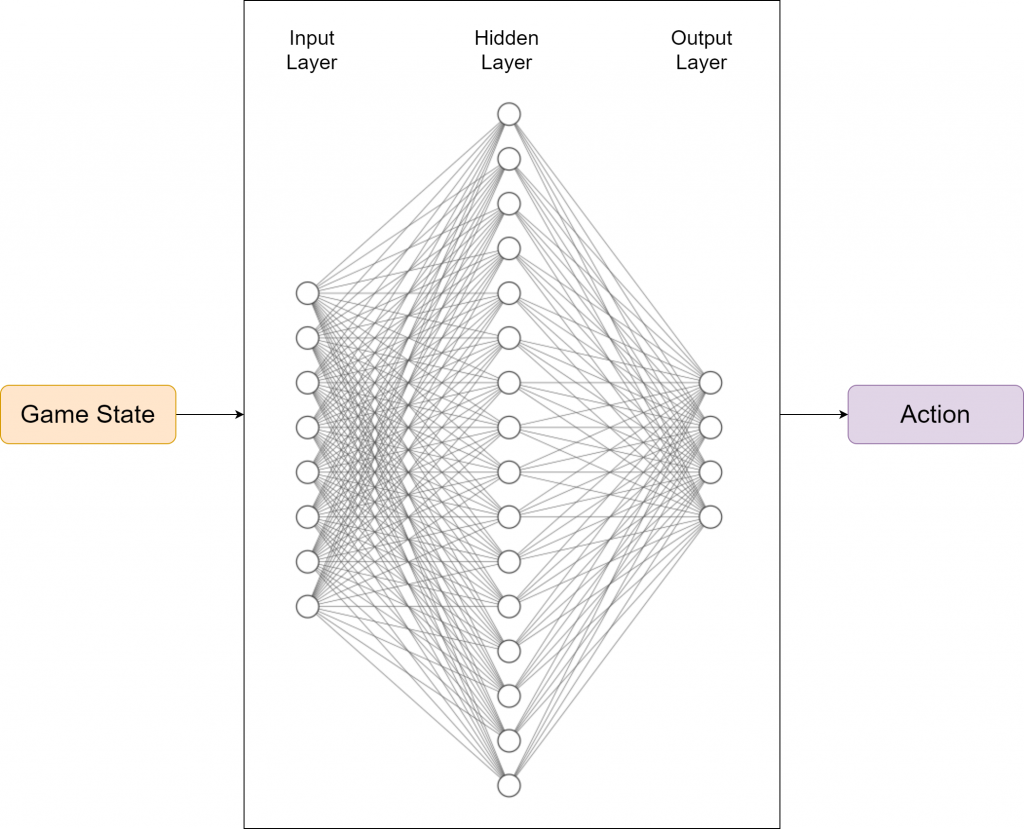
As explained previously, we utilize Deep Q-Learning as the backbone of our model, and the responsibility of the model is to inform the baby of the correct decision that must be made after each move. In other words, the model acts as the brain of the child, as the model helps the baby in making the critical decisions to eventually reach the target while avoiding the obstacles.
Inputs
The inputs to the model are provided as a vector of binary values to represent the following states.
- X1 - Whether the baby moves towards the top direction
- X2 - Whether the baby moves towards the right direction
- X3 - Whether the baby moves towards the bottom direction
- X4 - Whether the baby moves towards the left direction
- X5 - Whether the light source is to the top of baby
- X6 - Whether the light source is to the right of baby
- X7 - Whether the light source is to the bottom of baby
- X8 - Whether the light source is to the left of baby
Based on the input values, a vector of inputs is created as follows.
[X1, X2, X3, X4, X5, X6, X7, X8]
Architecture
For the model, we have utilized the input layer, a single hidden layer with 256 neurons, and finally an output layer to release the actions. ReLu is used as the activation function between the layers, and in future iterations, the deeper models will be tested to see how effective the model will be. In terms of the choice of the optimizer, while we have a number of choices, we decided to make use of Adam optimizer as it has found to be effective in most of the scenarios. On the other hand, we consider the Mean Squared Error (MSE) as the evaluation criteria, as we continuously attempt to minimize the MSE. The model requires several hyperparameters, and we have used the following hyperparameter values to start with: Learning Rate = 0.001, Batch Size = 1000, and Gamma = 0.9.
Outputs
The output defines the correct action that must be taken by the baby in order to maximize the benefits obtained by the baby. As such, the output represents the action space along with their probabilities that correspond to the maximization of rewards. An example is as follows.
[Q value for Top Move, Q value for Right Move, Q value for Bottom Move, Q value for Left Move]
Among the output Q values, the action with the highest Q value is chosen, and the action is accordingly taken by the baby.
Implementation
Based on the parameters given above, the neural network can be illustrated as follows. In this particular problem, we have 256 neurons in the hidden layer whereas the neurons corresponding to the input layer and output layer, are illustrated based on actual values.
The following file demonstrates the implementation of the model, using PyTorch.
model.py
import torch
import torch.nn as nn
import torch.optim as optim
import torch.nn.functional as F
import os
from datetime import datetime

VERSION = 1

class Linear_QNet(nn.Module):
    def __init__(self, input_size, hidden_size, output_size):
        super().__init__()
        self.linear1 = nn.Linear(input_size, hidden_size)
        self.linear2 = nn.Linear(hidden_size, output_size)

    def forward(self, x):
        x = F.relu(self.linear1(x))
        x = self.linear2(x)
        return x

    def save(self, n_games, best = False):
        model_folder_path = './model/v' + str(VERSION)
        date = datetime.today().strftime('%Y-%m-%d')
        if not os.path.exists(model_folder_path):
            os.makedirs(model_folder_path)
        if best:
            file_name = os.path.join(model_folder_path, 'best_' + str(date) + '_' + str(n_games) + '.pth')
        else:
            file_name = os.path.join(model_folder_path, str(date) + '_' + str(n_games) + '.pth')
        torch.save(self.state_dict(), file_name)

    def load(self, file_name = 'model.pth'):
        model_folder_path = './model'
        file_name = os.path.join(model_folder_path, file_name)

        if os.path.isfile(file_name):
            self.load_state_dict(torch.load(file_name))
            self.eval()
            print ('Loading existing state dict.')
            return True

        print ('No existing state dict found. Starting from scratch.')
        return False


class QTrainer:
    def __init__(self, model, lr, gamma):
        self.model = model
        self.lr = lr
        self.gamma = gamma
        self.optimizer = optim.Adam(model.parameters(), lr = self.lr)
        self.criterion = nn.MSELoss()

    def train_step(self, state, action, reward, next_state, done):
        state = torch.tensor(state, dtype=torch.float)
        next_state = torch.tensor(next_state, dtype=torch.float)
        action = torch.tensor(action, dtype=torch.long)
        reward = torch.tensor(reward, dtype=torch.float)

        if len(state.shape) == 1:
            # x > (1, x)
            state = torch.unsqueeze(state, 0) # Axis 0
            next_state = torch.unsqueeze(next_state, 0) # Axis 0
            action = torch.unsqueeze(action, 0) # Axis 0
            reward = torch.unsqueeze(reward, 0) # Axis 0
            done = (done, )

        # 1: Predicted Q values with the current state
        pred = self.model(state)

        target = pred.clone()
        for idx in range(len(done)):
            Q_new = reward[idx]
            if not done[idx]:
                # 2: Q_new = r + y * max(next_predicted_Q_value) -> Do this only if not done
                Q_new = reward[idx] + self.gamma * torch.max(self.model(next_state[idx]))
            target[idx][torch.argmax(action[idx]).item()] = Q_new

        self.optimizer.zero_grad()
        loss = self.criterion(target, pred)
        loss.backward()

        self.optimizer.step()
Game (Played by an Agent)
In order to accommodate the addition of Agent and Model, the game.py needs to be modified as shown below.
game.py
import pygame
import random
from enum import Enum
from collections import namedtuple
import math
import numpy as np

pygame.init()

font = pygame.font.Font('arial.ttf', 25)

# Possible directions of the Baby
class Direction(Enum):
    RIGHT = 1
    LEFT = 2
    UP = 3
    DOWN = 4

Point = namedtuple('Point', 'x, y')

#RGB Colours
WHITE = (255, 255, 255)
BLACK = (0, 0, 0)
GREEN1 = (107,142,35)
GREEN2 = (173,255,47)

BLOCK_SIZE = 30
SPEED = 60
NEGATIVE_SCORE_THRESHOLD = 30

class BabyRL():

    def __init__(self, w = 960, h = 720):
        self.w = w
        self.h = h

        # Initialize the Display
        self.display = pygame.display.set_mode((self.w, self.h))
        pygame.display.set_caption('Path Finder')
        self.clock = pygame.time.Clock()
        self.reset()

    def reset(self):
        # Initialize the game state and place the target
        self.direction = Direction.LEFT
        self.head = Point(self.w/2, self.h/2)
        self.head_prev = Point(self.w/2, self.h/2)

        self.score = 0
        self.target = None

        self._place_target()
        self.frame_iteration = 0

    def _place_target(self):
        # Place the target inside the window
        x = random.randint(0, (self.w - BLOCK_SIZE) // BLOCK_SIZE) * BLOCK_SIZE
        y = random.randint(0, (self.h - BLOCK_SIZE) // BLOCK_SIZE) * BLOCK_SIZE
        self.target = Point(x, y)

        # To ensure that the target does not get placed on the Baby
        if self.target == self.head:
            self._place_target()

    def play_step(self, action):

        # For each play_step, the number of frames must be iterated.
        self.frame_iteration += 1

        # Collect user input to catch the QUIT event. Unlike the game played by humans, we do not capture KEYDOWN inputs for determining the direction.
        # Instead, the computer must decide which action to take. As such, the "action" is a parameter of the play_step function.
        for event in pygame.event.get():
            if event.type == pygame.QUIT:
                pygame.quit()
                quit()

        # Move the Baby based on the "action" determined by the computer.
        # Previously, we used self.direction, which was determined by the human player.
        self._move(action)  # Update the head

        # Check if the game is over
        # If the game is over, a negative reward must be awarded to discourage the events of game over.
        reward = 0
        game_over = False
        if self.is_collision() or self.score < -NEGATIVE_SCORE_THRESHOLD:
            game_over = True
            reward = -10
            game_over_text = font.render("GAME OVER!", True, WHITE)
            game_over_text_rect = game_over_text.get_rect(center=(self.w/2, self.h/2))
            self.display.blit(game_over_text, game_over_text_rect)
            pygame.display.flip()
            return reward, game_over, self.score

        # If the Baby is moving away, penalize by deducting the score.
        if self._is_moving_away():
            self.score -= 5

        # If the Baby is getting close, award more scores.
        # Further, the Baby must be rewarded for attempting to get clos to the target.
        if self._is_moving_close():
            self.score += 1
            reward += 1

        # Place new target or move the Baby
        # If the Baby reaches the target, it must be rewarded accordingly.
        if self.head == self.target:
            self.score += 10
            reward += 10
            self._place_target()

        # Update UI and clock
        self._update_ui()
        self.clock.tick(SPEED)

        # Return if the game is over and score
        return reward, game_over, self.score

    def is_collision(self):
        # Does it hit the boundary?
        if (self.head.x > self.w - BLOCK_SIZE) or (self.head.x < 0) or (self.head.y > self.h - BLOCK_SIZE) or (self.head.y < 0):
            return True
        return False

    def _is_moving_away(self):
        prev_distance = math.hypot(self.head_prev.x - self.target.x, self.head_prev.y - self.target.y)
        current_distance = math.hypot(self.head.x - self.target.x, self.head.y - self.target.y)
        if current_distance > prev_distance:
            return True
        return False

    def _is_moving_close(self):
        prev_distance = math.hypot(self.head_prev.x - self.target.x, self.head_prev.y - self.target.y)
        current_distance = math.hypot(self.head.x - self.target.x, self.head.y - self.target.y)
        if current_distance > prev_distance:
            return False
        return True

    def _move(self, action):
        # [Up, Right, Down, Left]

        if np.array_equal(action, [1, 0, 0, 0]):
            new_direction = Direction.UP
        elif np.array_equal(action, [0, 1, 0, 0]):
            new_direction = Direction.RIGHT
        elif np.array_equal(action, [0, 0, 1, 0]):
            new_direction = Direction.DOWN
        elif np.array_equal(action, [0, 0, 0, 1]):
            new_direction = Direction.LEFT

        self.direction = new_direction

        x = self.head.x
        y = self.head.y
        self.head_prev = Point(x, y)

        if self.direction == Direction.RIGHT:
            x += BLOCK_SIZE
        elif self.direction == Direction.LEFT:
            x -= BLOCK_SIZE
        elif self.direction == Direction.DOWN:
            y += BLOCK_SIZE
        elif self.direction == Direction.UP:
            y -= BLOCK_SIZE

        self.head = Point(x, y)

    def _update_ui(self):
        self.display.fill(BLACK)

        # Drawing the Baby
        pygame.draw.rect(self.display, GREEN1, pygame.Rect(self.head.x, self.head.y, BLOCK_SIZE, BLOCK_SIZE))
        pygame.draw.rect(self.display, GREEN2, pygame.Rect(self.head.x + 6, self.head.y + 6, 18, 18))

        # Drawing the Target
        pygame.draw.rect(self.display, WHITE, pygame.Rect(self.target.x, self.target.y, BLOCK_SIZE, BLOCK_SIZE))

        text = font.render("Score: " + str(self.score), True, WHITE)
        self.display.blit(text, [0, 0])
        pygame.display.flip()
Now you have a game where the computer learns gradually to reach the target.
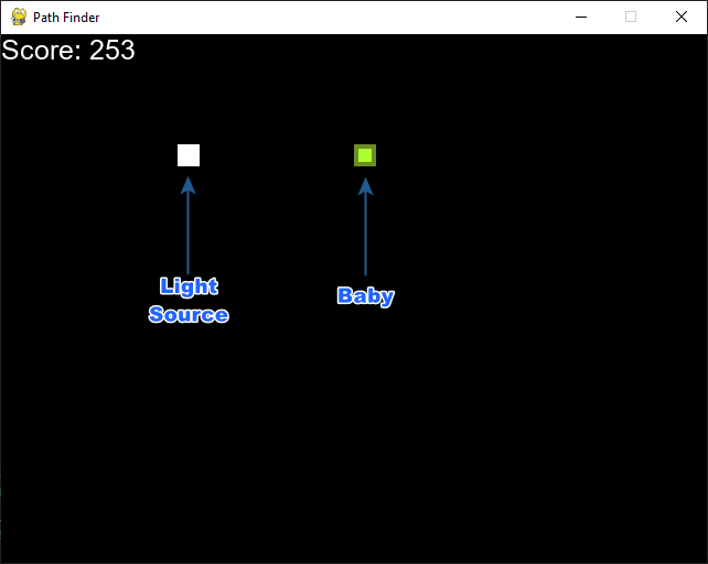
Demonstration
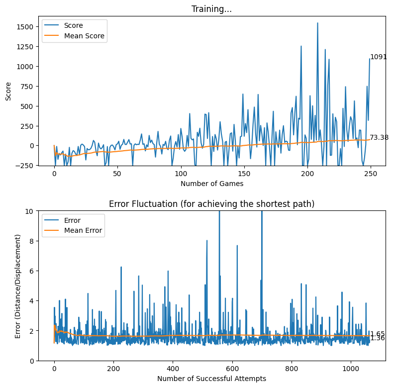
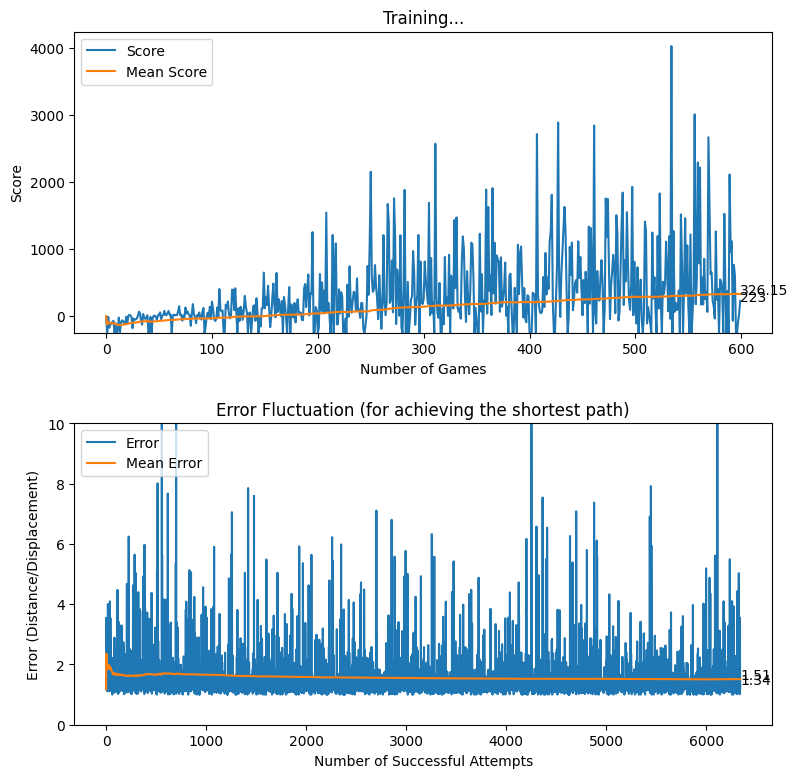
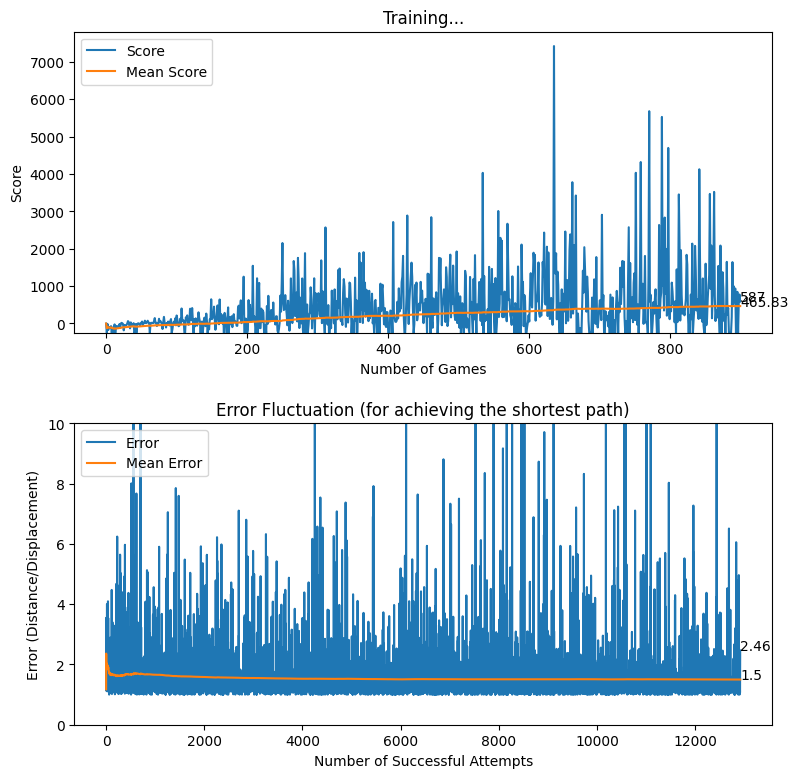
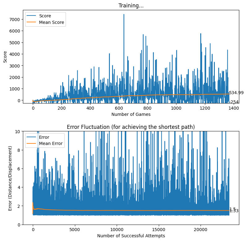
After creating the game as explained in the previous sections, we actually trained our model (baby) to see if it can actually recognize the patterns, self learn and eventually chase the light source. And, we obviously made it possible! With enough training and time, the model self learns the optimal actions, and it is evident from the small video clips shown below.
As shown above, the computer (baby) initially struggles to finds the way towards the target, but with gradual training, it learns the pattern and attempts to maximize the reward. After some hours of training, it becomes unstoppable, and it rarely hits the obstacles (in this case, the walls).
In this article, we brought you a small demonstration to show the power of reinforcement learning, and to show you how we can leverage the absolute power of reinforcement learning for optimizing our own tasks. Nonetheless, we believe that this is an area of research that can be effectively applied to most of the domains, and we believe that we can prosper in this area with novel applications with the power of machine learning.
Feature Additions
In the previous attempt, our goal was to create a proof of concept to ideally demonstrate that the computer can actually SELF LEARN with adequate training. However, we did not want to just stop our quest at the previous milestone. Instead, we focused on improving the environment and the model to see how the baby will self learn under challenging circumstance. Despite all our attempts, the we ensured that the computer achieves self learning with adequate training, and here is a demonstration of how we enhanced the gameplay with feature additions to both the game and the baby.
Widening the Action Space
The action space in the previous attempt was limited to four (UP, RIGHT, DOWN, LEFT). However, we decided to widen the action space by incorporating more moves to the baby, as it gives the baby more freedom to move inside the plain. As a result, we created 19 distinct actions that the baby can effectively take after each action.
As such, the following list of actions were made possible.
| Action | Description |
|---|---|
| 90L-1B | 1 Unit Distance to 90 Degrees Left |
| 80L-1B | 1 Unit Distance to 80 Degrees Left |
| 70L-1B | 1 Unit Distance to 70 Degrees Left |
| 60L-1B | 1 Unit Distance to 60 Degrees Left |
| 50L-1B | 1 Unit Distance to 50 Degrees Left |
| 40L-1B | 1 Unit Distance to 40 Degrees Left |
| 30L-1B | 1 Unit Distance to 30 Degrees Left |
| 20L-1B | 1 Unit Distance to 20 Degrees Left |
| 10L-1B | 1 Unit Distance to 10 Degrees Left |
| S-1B | 1 Unit Distance Straight |
| 10R-1B | 1 Unit Distance to 10 Degrees Right |
| 20R-1B | 1 Unit Distance to 20 Degrees Right |
| 30R-1B | 1 Unit Distance to 30 Degrees Right |
| 40R-1B | 1 Unit Distance to 40 Degrees Right |
| 50R-1B | 1 Unit Distance to 50 Degrees Right |
| 60R-1B | 1 Unit Distance to 60 Degrees Right |
| 70R-1B | 1 Unit Distance to 70 Degrees Right |
| 80R-1B | 1 Unit Distance to 80 Degrees Right |
| 90R-1B | 1 Unit Distance to 90 Degrees Right |
The resulting action space is demonstrated by an array of binary values as shown below.
[90L-1B, 80L-1B, 70L-1B, 60L-1B, 50L-1B, 40L-1B, 30L-1B, 20L-1B, 10L-1B, S-1B, 10R-1B, 20R-1B, 30R-1B, 40R-1B, 50R-1B, 60R-1B, 70R-1B, 80R-1B, 90R-1B]
For instance, if the model decides that the baby must turn right by 30 degrees, the following array will be provided as the action space.
[0, 0, 0, 0, 0, 0, 0, 0, 0, 0, 0, 0, 1, 0, 0, 0, 0, 0, 0]
With this feature addition, our intention was to provide more freedom to the baby to move along with 2D plain rather than restricting the baby to just four possible steps. In this process, we were also careful enough to consider the moving direction angle as a variable in order to maintain the heading direction of the baby. This allows us to properly guide the baby towards the action determined by the neural network.
UI Enhancement - Adding Trails
So far in our development, it was not possible for us to see the trails created by the baby. Therefore, we decided to add the trail created by the baby, alongside the optimum trail (displacement) which is demonstrated in a different colour. While this modification does not yield any enhancement to the model or the environment, it definitely provides a visually appealing scene that allows us to see and understand the movements made by the baby. The following video demonstrates the UI enhancement and the wide range of actions that can be performed by the baby. Please note that the video demonstrates a model which is at the very early stages of a training session.
In this video, the BLUE colour trail represents the trail of the baby before reaching the destination whereas the WHITE colour line represents the displacement between baby’s initial position and the expected destination.
Enriching the State Space
The state space effectively acts as the input layer of the underlying neural network that powers the whole process of decision making. Up to this stage, the neural network received the inputs in the following form.
- X1 - Whether the baby moves towards the top direction
- X2 - Whether the baby moves towards the right direction
- X3 - Whether the baby moves towards the bottom direction
- X4 - Whether the baby moves towards the left direction
- X5 - Whether the light source is to the top of baby
- X6 - Whether the light source is to the right of baby
- X7 - Whether the light source is to the bottom of baby
- X8 - Whether the light source is to the left of baby
Inputs = [X1, X2, X3, X4, X5, X6, X7, X8]
While the above inputs are acceptable to the neural network, we realized that the enrichment of the state space can potentially improve the decision making process of the neural networks. From the perspective of human decision making, it is obvious that the human is capable of making more informed decisions if more prior knowledge is available. In the same manner, we decided to include few additional, yet important parameters to the state space with the intention of supporting the neural network.
At a given moment, the baby can effectively get the information if the baby is nearby a danger. From a machine perspective, this kind of information can be gathered with the use of sensors. Essentially, since the baby has to make a choice among 19 possible actions, we decided to let the baby calculate the potential danger of making such decisions, and include the danger statuses as the inputs to the neural network. Thus, the baby artificially makes moves each of the 19 moves, and check if any of such moves result in a collision with the wall. If it is detected that a collision is imminent, the input layer is updated in the form of binary values. Therefore, we can get the input layer as follows.
- X1 - Whether the baby collides if baby makes a left turn of 90 degrees with a displacement of a unit distance
- X2 - Whether the baby collides if baby makes a left turn of 80 degrees with a displacement of a unit distance
- X3 - Whether the baby collides if baby makes a left turn of 70 degrees with a displacement of a unit distance
- X4 - Whether the baby collides if baby makes a left turn of 60 degrees with a displacement of a unit distance
- X5 - Whether the baby collides if baby makes a left turn of 50 degrees with a displacement of a unit distance
- X6 - Whether the baby collides if baby makes a left turn of 40 degrees with a displacement of a unit distance
- X7 - Whether the baby collides if baby makes a left turn of 30 degrees with a displacement of a unit distance
- X8 - Whether the baby collides if baby makes a left turn of 20 degrees with a displacement of a unit distance
- X9 - Whether the baby collides if baby makes a left turn of 10 degrees with a displacement of a unit distance
- X10 - Whether the baby collides if baby goes straight with a displacement of a unit distance
- X11 - Whether the baby collides if baby makes a right turn of 10 degrees with a displacement of a unit distance
- X12 - Whether the baby collides if baby makes a right turn of 20 degrees with a displacement of a unit distance
- X13 - Whether the baby collides if baby makes a right turn of 30 degrees with a displacement of a unit distance
- X14 - Whether the baby collides if baby makes a right turn of 40 degrees with a displacement of a unit distance
- X15 - Whether the baby collides if baby makes a right turn of 50 degrees with a displacement of a unit distance
- X16 - Whether the baby collides if baby makes a right turn of 60 degrees with a displacement of a unit distance
- X17 - Whether the baby collides if baby makes a right turn of 70 degrees with a displacement of a unit distance
- X18 - Whether the baby collides if baby makes a right turn of 80 degrees with a displacement of a unit distance
- X19 - Whether the baby collides if baby makes a right turn of 90 degrees with a displacement of a unit distance
- X20 - Whether the baby moves towards the top direction
- X21 - Whether the baby moves towards the right direction
- X22 - Whether the baby moves towards the bottom direction
- X23 - Whether the baby moves towards the left direction
- X24 - Whether the light source is to the top of baby
- X25 - Whether the light source is to the right of baby
- X26 - Whether the light source is to the bottom of baby
- X27 - Whether the light source is to the left of baby
Inputs = [X1, X2, X3, X4, X5, X6, X7, X8, X9, X10, X11, X12, X13, X14, X15, X16, X17, X18, X19, X20, X21, X22, X23, X24, X25, X26, X27]
Working with Obstacles
Our next attempt was to make it difficult for the baby to find the way towards the destination, by adding obstacles. This was an attempt by us to check if the baby can self learn to effectively avoid the obstacles and finally reach the destination. From a practical point of view for a machine, we believe that this is an important hurdle to get past. Initially, we worked with a single block of obstacle and trained the model to see if it can do the job for us. Interestingly, after hours of training, the baby does avoid the collision with obstacles and reach the target. You may view the video shown below to see how it actually performs.
As the next step, we decided to add another block of obstacle to observe the behavior of the training agent. As expected, the baby learned to avoid the obstacles while reaching the destination, as shown in the following videos.
Troubleshooting - Discouraging Unusual Actions
In the previous training iterations, you must have noticed an unusual behaviour depicted by the child. What we mean by the unusualness here is that the baby tends to move around the same path multiple times while attempting to reach the destination. In a real world scenario, this kind of a behaviour is unacceptable as it could lead to a waste of resources. As a solution, we thought that it would be appropriate to discourage such repeated and unusual actions by awarding a penalty for such occurrences. Thus, we introduced the following changes.
The game is instructed to keep track of the last n number of coordinates (positions) of the baby in a queue. As a result, every time the baby makes a move, the queue gets updated while preserving the last n number of traversed positions of the baby. Additionally, if it is found that the baby’s current position is nearby one of the last n traversed positions, the baby is awarded a negative reward. For implementation purposes, we considered n = 100 and the nearness is determined by considering the 2 x 2 (pixel²) block of each of the traversed points. The following pseudocode and the diagram should assist you in understanding the logic behind the negative reward awarding system.
current_position_x = baby.x
current_position_y = baby.y

for traversed_point in traversed_points:
  if ((current_position_x < traversed_point.x + 1 ) and (current_position_x > traversed_point - 1)) and ((current_position_y < traversed_point.y + 1) and (current_position_y > traversed_point.y - 1)):
    reward = -50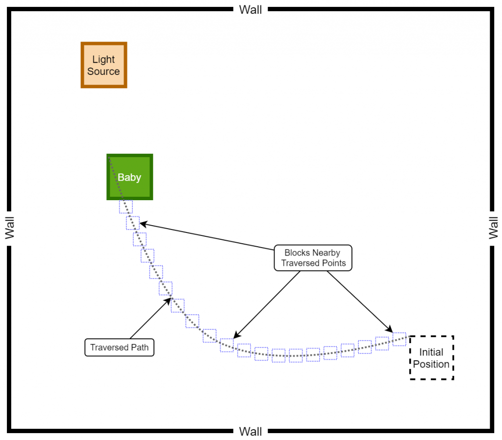
Rewarding based on Displacement Trail
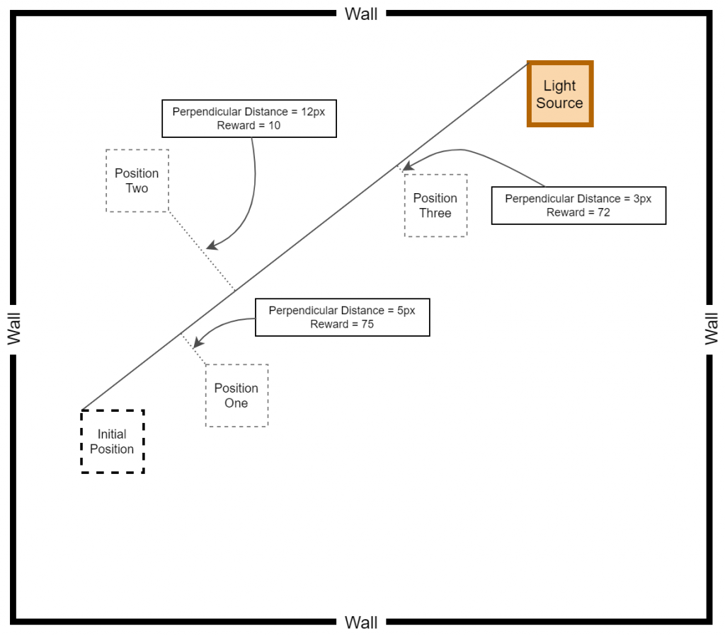
After many training sessions, we realized that the baby can actually self learn even with the availability of a much wider action space. However, so far, we have utilized the base rewarding mechanism explained here [hyperlink to appear here]. Additionally, we have introduced a negative rewarding mechanism for discouraging sub-optimal actions as explained in the previous section. Nonetheless, with the intention of improving the quality of actions made by the baby, we experimented with a new rewarding system where the baby is rewarded more for staying close to the displacement line. The thought process behind the implementation of this rewarding mechanism was that we wanted to encourage the baby to follow the shortest possible path while achieving the quest of reaching the destination.
reward = 0
game_over = False
current_position_x = baby.x
current_position_y = baby.y

if (baby collides with a wall) or (score < NEGATIVE_SCORE_THRESHOLD):
    game_over = True
    reward = -100

# If the baby is moving away, penalize by rewarding negatively.
if (baby moves away from the light source):
    reward = -20

# The baby must be rewarded for attempting to get close to the target.
if (baby gets close to the light source):
    # Calculate the perpendicular_distance between baby and the displacement line (between initial position and destination)
    reward = 75 - perpendicular_distance
    if reward >= 70:
      reward = reward
    else:
      reward = 10

# Discouraging sub-optimal actions
for traversed_point in traversed_points:
  if ((current_position_x < traversed_point.x + 1 ) and (current_position_x > traversed_point - 1)) and ((current_position_y < traversed_point.y + 1) and (current_position_y > traversed_point.y - 1)):
    reward = -50

# If the baby reaches the target, baby must be rewarded accordingly.
if (baby reaches light source):
    reward = 100
As explained above, the baby is heavily rewarded if the baby manages to stay within a perpendicular distance of 5 pixels on either side of the displacement line. In other cases, although the reward is positive, a relatively less reward is awarded for attempting to get close to the target. The following diagram provides a better understanding of how the displacement based rewarding mechanism is implemented.
After applying the aforementioned rewarding system, we observed that the baby attempts to move closer to the displacement line while reaching the target. We further observed that the as baby learns, the obstacles (walls) are avoided to the best effect, thus the game over states occur rarely.
Rewarding based on Optimum Future Moves (two levels)
In the previous section, we experimented with a reward mechanism that makes the baby focus on staying closer to the displacement line. Since we were able to get excellent results from the displacement-based reward system, it was decided to experiment with another approach where the baby is rewarded for taking optimum actions by searching through the future optimal action spaces. In this case, we started off by considering the action spaces only up to two levels because this is more of a brute-force approach where we check each and every possibility before making a move. In the long run, this kind of an approach can be infeasible due to the amount of processing power it needs to train the agent.
In this approach, as explained previously, the quality of potential future moves up to two levels are explored and the baby is rewarded heavily if the action taken by the neural network is a good move. Thus, the reward for each move depends on the optimality of the future moves.
Note: The following logic has been implemented using two different for-loops. However, this code can be optimized by using a recursive function.
def get_move_based_reward(self, action):
    # Maintaining a dictionary to store the distances between potential future moves, and the destination
    self.moves = defaultdict(dict)

    # Current moving angle is the last angle taken by the baby
    current_angle = self.angle_prev

    # Getting the current position of the baby
    head_position = self.head

    # Iterating through first level of future moves
    for angle in range(90,-100,-10):

        # Setting the future angle
        first_level_angle = current_angle
        first_level_angle += math.radians(angle)

        # Imaginarily placing the baby on the possile move of the first level
        x = head_position.x + JUMP_DISPLACEMENT*math.cos(first_level_angle)
        y = head_position.y - JUMP_DISPLACEMENT*math.sin(first_level_angle)
        first_level_head_position = Point(x, y)

        # Iterating through the second level of future moves
        for second_angle in range(90, -100, -10):

            # Setting up the second level future angle
            second_level_angle = first_level_angle
            second_level_angle += math.radians(second_angle)

            # Imaginarily placing the baby on the possile move of the second level
            second_x = first_level_head_position.x + JUMP_DISPLACEMENT*math.cos(second_level_angle)
            second_y = first_level_head_position.y - JUMP_DISPLACEMENT*math.sin(second_level_angle)
            second_level_head_position = Point(second_x, second_y)

            # Getting the distance between the destination and the position of the terminal level of tree
            distance_to_target = math.hypot(second_level_head_position .x - self.target.x, second_level_head_position.y - self.target.y)

            # Updating the dictionary
            if self.moves.get(str(angle)) is None:
                self.moves[str(angle)] = distance_to_target
            else:
                if self.moves[str(angle)] > distance_to_target:
                    self.moves[str(angle)] = distance_to_target

    # Sorting the dictionary of moves
    self.moves = dict(sorted(self.moves.items(), key = lambda item: item[1]))

    # Action <=> Angle Mapping
    # With this mapping, we get the angle suggested by the neural network as the next move.
    # As such, action_angle is the angle suggested by the neural network.
    action_index = action.index(1)
    action_angle = None
    angle_iterator = 0
    for angle in range(90, -100, -10):
        if angle_iterator == action_index:
            action_angle = angle
            break
        angle_iterator += 1

    # Calculating the distance between previous (last) actual position of baby and the destination
    # The calculated distance is then compared with the distances of potential future moves, and
    # we get rid of potential future moves that are getting away from the target.
    # This gives us a ranked list of "good" potential future moves.
    prev_distance = math.hypot(self.head_prev.x - self.target.x, self.head_prev.y - self.target.y)
    self.moves = dict((k, v) for k, v in self.moves.items() if v <= prev_distance)

    # Checking if the action_angle (angle or move suggested by the neural network) exists in the
    # list of "good" moves. The baby is then rewarded based on the action.
    if str(action_angle) in self.moves:
        rank = list(self.moves).index(str(action_angle))
        reward = (75/len(self.moves))*(len(self.moves) - rank)
    else:
        reward = 0
    return int(reward)
While the above reward function works as expected, we later realized that the the final reward calculation retains a sense of biasness if the the number of “good” moves is less. Therefore, in the next iteration of our development, we introduced a slight change as follows.
   # Checking if the action_angle (angle or move suggested by the neural network) exists in the
    # list of "good" moves. The baby is then rewarded based on the action.
    if str(action_angle) in self.moves:
        rank = list(self.moves).index(str(action_angle))
        if rank < 5:
          reward = 75 - rank*5
        else:
          reward = 10
    else:
        reward = 0
Working with a grid of obstacles
In the section "Working with Obstacles", we discussed about the inclusion obstacles to make it difficult for the baby to learn the end goals. Nevertheless, it did not end up becoming a hurdle for the baby as the baby comfortably managed to avoid the obstacles. However, we utilized only two obstacles at a time for the sake of simplicity. As per our next set of experiments, it was decided to include a grid of obstacles to make it look like a maze, as shown in the following diagram.
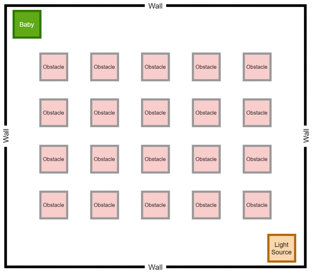
Surprisingly (or not surprisingly), after some hours of training, the baby managed to find his/her way towards the destination while avoiding the grid of obstacles. As we had experimented with two types of rewarding mechanisms (displacement-based and optimum future moves-based), the game was trained using both rewarding systems separately, and we certainly received excellent results in both types of rewarding systems.
Optimum Future Moves based Reward
In this case, the optimum future moves were implemented, but compared to the explanation given previously, this time around, we went ahead with three levels of depth search instead of two levels. The results are impressive as shown in the following video clips.
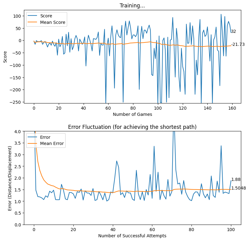
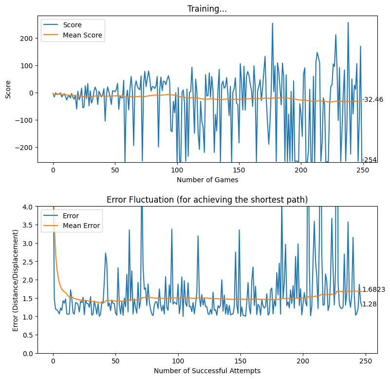
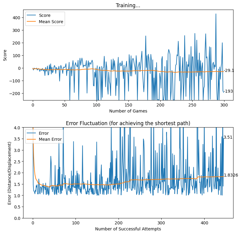
Displacement based Reward
In a similar manner with the grid of obstacles, the game was trained with the displacement-based reward system and the results are illustrated below.
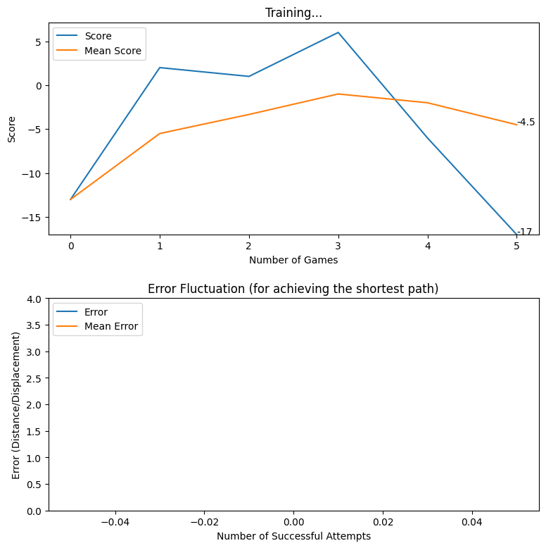
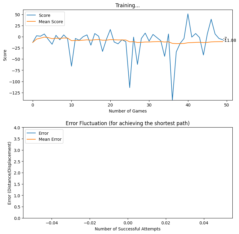
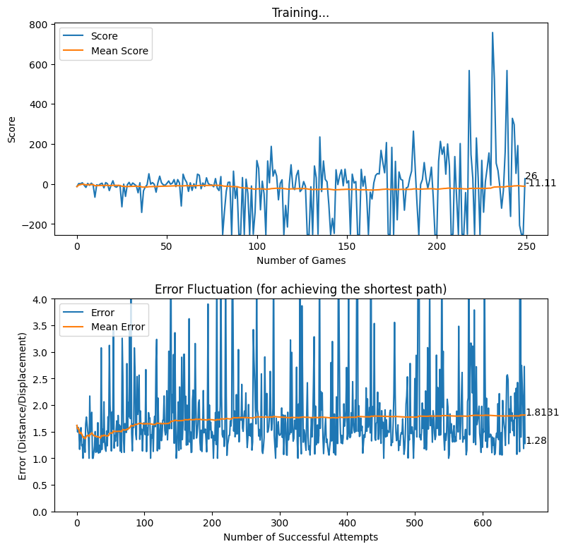
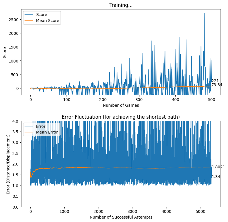
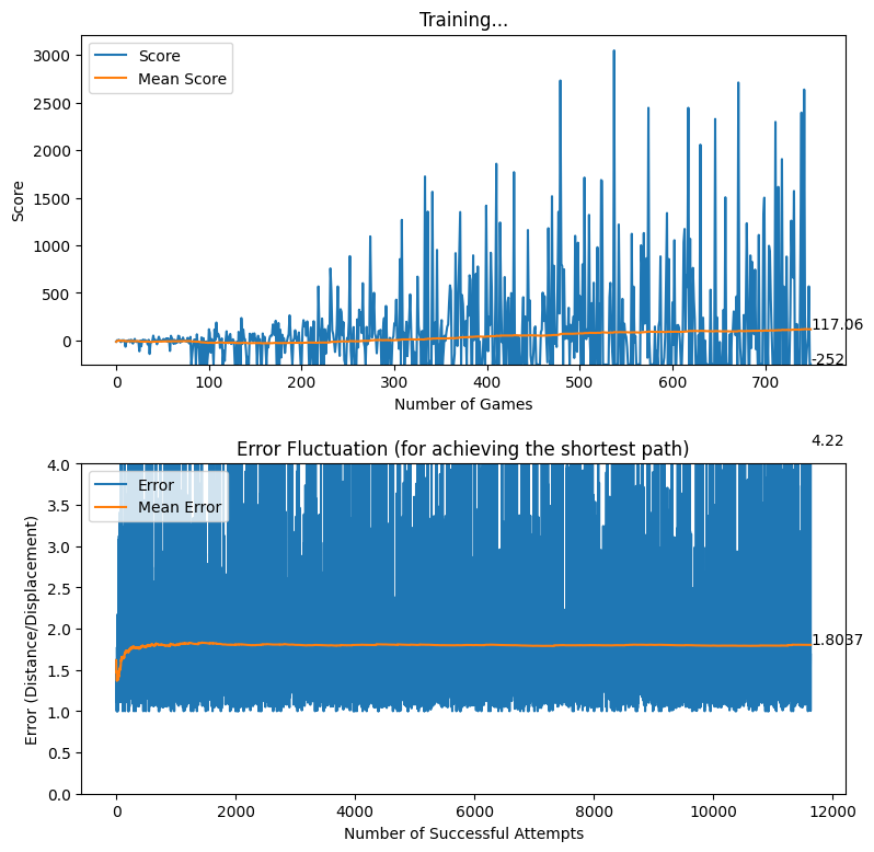
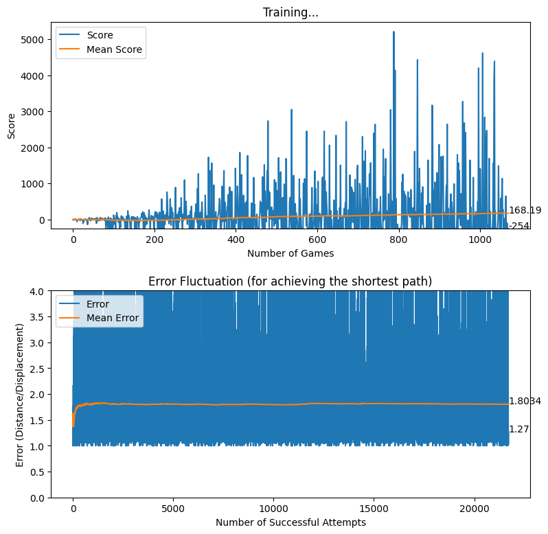
A CNN Approach for Recognizing Traffic Signs
Deep Learning is an interesting and a unique field of study that has attracted the worldwide attention over the past few years at a rapid pace. The rate at which the digitalized systems have been generating data for over a decade, has become one of the major reasons for creating an abundance of data. As a result, the availability of data provided a brand new perspective for the researchers to look at Artificial Intelligence and its branches, in a different way. Additionally, the gradual enhancement of hardware resources resulted in offering much improved computational resources for the deep learning researchers to make use of data efficiently. Therefore, the combination of data and modern computational resources, was able to create a platform for the researchers to thrive on, and the result is a highly motivated deep learning community that continues to contribute towards the growth of deep learning using novel approaches. Computer vision is a research area that has benefitted largely from the rise of deep learning, and it is evident from the amount of research studies carried out in computer vision with deep learning.
While there are many specific applications of computer vision, the uses of deep learning in traffic/road related applications, is an interesting application since it directly affects the improvement of vehicular automation. Although the field of vehicular automation is on the verge of reaching greater heights, as evident from Tesla’s Autopilot feature (and similar implementations from other major automobile manufacturers), understanding the fundamentals of deep learning remains an integral part for those who are interested in exploring the capabilities of deep learning. In this article, we focus on bringing you a primer for understanding how the nuts and bolts of deep learning can effectively improve the metrics that measure the success of a specific application that targets traffic signs. Thus, our attempt is to explore the process of developing a traffic sign recognizer using the concepts of deep learning.
We have structured the article in way that allows you to easily move to the desired section with ease. Initially, we explain the Background behind the problem before coming up with an Exploratory Data Analysis for the dataset which we utilized. Afterwards, the Deep Learning Workflow provides a high-level overview of the procedure followed by us, and then we place our emphasis on creating a suitable Input Pipeline for preparing the data to meet the requirements of the Models explained in the subsequent section. Finally, we examine the performance of the developed model, before capping the article off by deploying it as a readymade model which can be tested by yourself using an interactive interface. Sounds interesting, huh?
Background
The Problem
A brief writeup on the actual problem that we are attempting to address. In our context, the broader problem is to check the possibility of recognizing the traffic signs via the concepts of computer vision.
What will straightly come to your mind if you are asked to think of a main road in any part of the world? Obviously, the pedestrians and vehicles should greet your mind as they make the roads busy, thanks to the continuous movements made by them. The clutters of vehicles and pedestrians can certainly lead to unpleasant outcomes, and as a result, standardized road rules have been set up by the authorities to minimize the clutters and to streamline the traffics in a structured manner. Since the drivers and pedestrians are supposed to obey the rules, having assistive signs/lights can definitely help both the drivers and pedestrians to ensure that the road is a safe environment for everyone.
This is where the importance of traffic signs, comes into the frame to act as guidelines for both drivers and pedestrians. While the traffic signs are supposed to be understood by human vision, it is interesting to if the same phenomenon can be emulated using computer vision. In this article, we attempt to address a basic problem, in which we check the possibility of recognizing the traffic signs via the concepts of computer vision.
The Aim (and objectives)
In a broader context, our aim is to develop a recognizer that correctly classifies a given traffic sign image to determine its class, using the concepts of deep learning in computer vision. It is expected to achieve the aim by methodically following the objectives given below.
- Exploring the health of the dataset by performing an Exploratory Data Analysis
- Preprocessing the data for building the input pipeline
- Defining a suitable methodology that iteratively improves the performance of the model.
- Testing the performances on unseen datasets.
- Developing a tool for allowing the user to self-test the capabilities of the developed model.
The Dataset
As we explained in the Introduction section, datasets play a pivotal role in the development of a deep learning based solution. Fortunately, there are freely available datasets for achieving our requirement. Therefore, we used the German Traffic Sign Recognition Benchmark (GTSRB) dataset provided by the Institut für Neuroinformatik. The dataset has been initially provided as a multi-class classification challenge at the International Joint Conference on Neural Networks (IJCNN) 2011.
Exploratory Data Analysis
The Exploratory Data Analysis (EDA) is a common component that provides a representation of the original dataset using descriptive statistical methods with the aid of relevant plots. For more information, refer the following link:
What is Exploratory Data Analysis?
Once we downloaded the ZIP file from the source given above, we came across datasets corresponding to three distinct categories inside the ZIP archive: Train, Test, and Meta. The images related to the Train dataset were stored inside the Train folder where separate sub-folders had been created to organize the Train images under different class labels. In contrast, the images related to the Test dataset were directly inside a folder named Test. The Meta folder was composed of computer-illustrated images to represent each class label and few of the images from all three categories are given below. Additionally, the archive contained three annotated Comma Separated Files (CSV) named Train.csv, Test.csv, and Meta.csv. The composition of each CSV file, is further discussed within this section in the following paragraphs.
Train
Sample Image from the Dataset
Number of Images
In order to explore the number of available images in the Train dataset, the Train.csv file can be analyzed. The Pandas library in Python is a useful tool for dealing with CSV files by including the data into a Dataframe. Based on the results, the dataset contained 39,209 images.
Number of Classes
The dataset consists of images corresponding to 43 classes, numbered sequentially from 0 to 42.
Class Distribution
The following figure represents the class distribution of the Train dataset.
Structure of Data
Altogether, the Train.csv file contains the following list of important fields which can be utilized as per the requirements [Ref: German Traffic Sign Benchmarks ]
- Width: The width of the image in pixels
- Height: The width of the image in pixels
- Roi.X1: The X-coordinate of top-left corner of traffic sign bounding box
- Roi.Y1: The Y-coordinate of top-left corner of traffic sign bounding box
- Roi.X2: The X-coordinate of bottom-right corner of traffic sign bounding box
- Roi.Y2: The Y-coordinate of bottom-right corner of traffic sign bounding box
- ClassId: The actual class label
Test
The annotated file for the Test dataset (Test.csv) also follows a layout similar to the Train.csv.
Sample Images from the Dataset

Number of Images
The Test dataset consists of 12,630 images as per the actual images in the Test folder and as per the annotated Test.csv file.
Number of Classes
As expected, The Test dataset also consists of images corresponding to 43 classes, numbered sequentially from 0 to 42.
Class Distribution
The following figure represents the class distribution of the Test dataset.
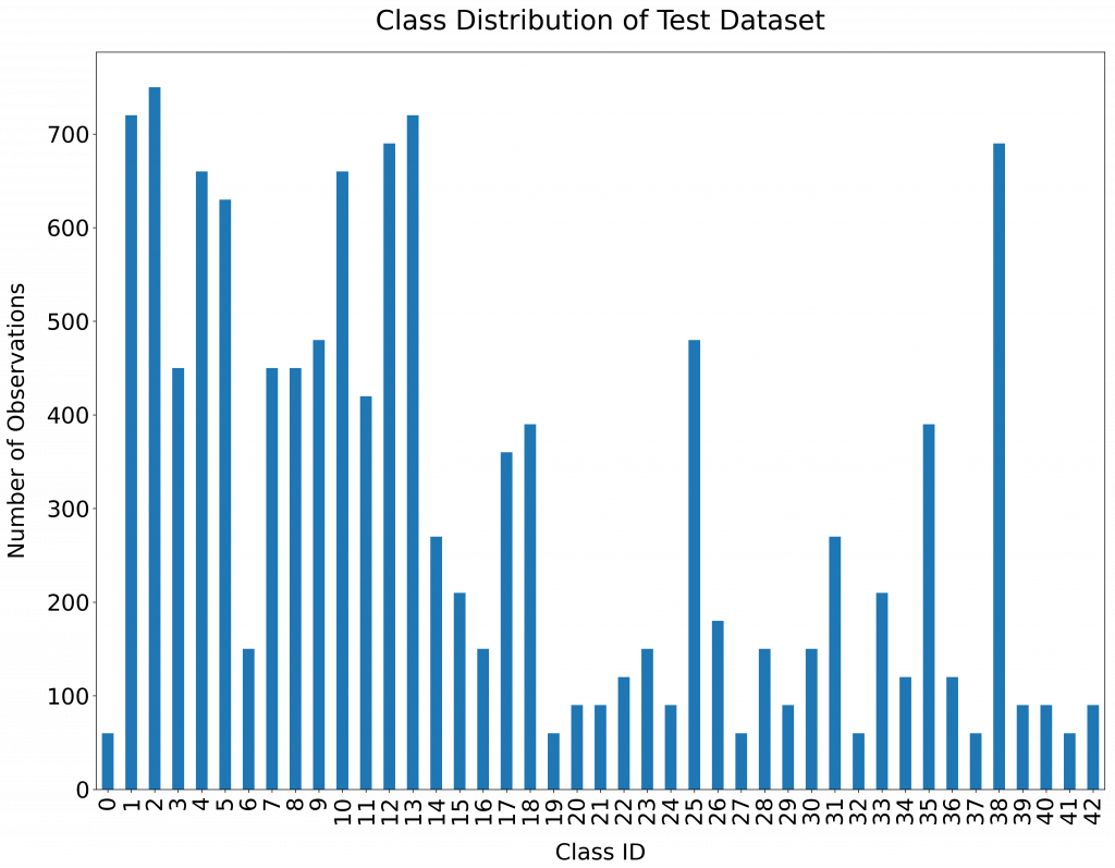
Meta

The Meta Dataset, along with the Meta.csv has been provided as a guideline to represent the actual images and the related Class labels.
The Deep Learning Workflow
Here, we will add a high level diagram for explaining the iterative workflow that we follow throughout the model development/improvement process. The diagram will represent the usual Machine/Deep Learning workflow, with specific customizations to cater the expected outcomes of our case study.
Over the years, the machine learning community has adopted a certain workflow that keeps them in the hunt for the reaching the desired aims and objectives. The following figure depicts the workflow which we usually follow in the process of developing machine/deep learning applications. In reality, deep learning is a highly iterative process that requires the developers to keep experimenting until the target objectives are achieved.
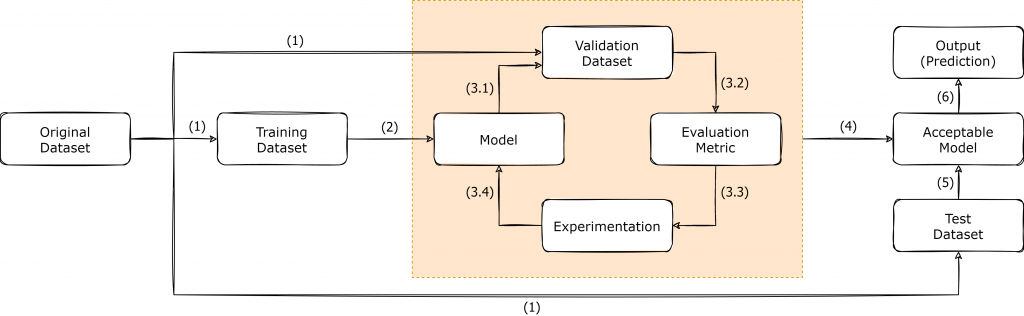
As shown in the above figure, once we have a dataset which is suitable to be applied for a deep learning task, the dataset is usually split into three subsets, known as Training Dataset, Validation Dataset and Test Dataset. The splitting process may vary, depending on the original dataset that you have, and in the context of GTSRB dataset, the authors had provided both the Training Dataset and Test Dataset separately. Since the Validation Dataset is not available in GTSRB dataset, it is up to the developers to decide the best possible way forward for creating a Validation dataset, depending on the application.
Once the Train/Validation/Test split is finalized, the Training Dataset is utilized for training the initial model, as shown in Step (2). The creation of the model initiates the iterative cycle where the model is tested against the Validation dataset to obtain the necessary evaluation metric. Based on the result of the evaluation metric, the developers are supposed to keep on experimenting and form a new model and follow the same cycle, until a model with a viable evaluation metric result is obtained. After the finalization of a model, it is considered as the Acceptable Model [Step (4)]. The Test Dataset consists of real-world data that the model has not previously seen and it provides us the opportunity to Test the created model against real-world data to actually see how it would eventually perform on the production run.
The Input Pipeline
In this section, the focus will be placed on the explaining the preprocessing steps which we followed, before the development of models.
For instance, the process of preparing Train/Validation/Test/StreetViewTest datasets, is explained, along with the other normalization steps taken during the process
In this section, we focus on the preparation of our original datasets according to a standard formats used in the process of practicing deep learning. Therefore, the preparation of the input pipeline can be illustrated in two separate steps where the first step is to prepare Training, Validation and Test datasets from the originally available data. Subsequently, we dive into the additional task of normalizing the inputs before sending them through the training cycle.
Initialization
Since this is the beginning of the code, first of all, it is required to import the necessary libraries which are required throughout the implementation.
import numpy as np
import pandas as pd
import matplotlib.pyplot as plt
import cv2
import tensorflow as tf
from PIL import Image
import keras
import os
from sklearn.model_selection import train_test_split
from tensorflow.python.keras import regularizers
Usually, when we deal with images, we deal with the array representations of the respective images, rather than working with the usually known JPEG or PNG (or any other image format) formats. The following code snippet shows how we load and convert the images to arrays from the originally available Train and Test image datasets. In the conversion job, we also place emphasis on making all the observations have the same shape when it comes to the representation of resolution of each observation. Therefore, each image is resized to have a resolution of 30x30 before being converted to a numpy array.
# Loading the Train Dataset
train_data = []
train_labels = []
basedir = "../Datasets/gtsrb"
classes = 43

for i in range(classes):
    path = os.path.join(basedir,'train',str(i))
    images = os.listdir(path)

    for j in images:
        print("Class: " + str(i) + " - Image: " + str(j))
        image = Image.open(path + '\\'+ j)
        image = image.resize((30,30))
        image = np.array(image)
        train_data.append(image)
        train_labels.append(i)

train_data = np.array(train_data)
train_labels = np.array(train_labels)

# Loading the Test Dataset

image_paths = []
test_data=[]
test_file_path = os.path.join(basedir, 'Test.csv')

Y_test_df = pd.read_csv(test_file_path)
Y_test_orig = Y_test_df["ClassId"].values

for short_path in Y_test_df["Path"]:
    image_paths.append(os.path.join(basedir, short_path))

for img in image_paths:
    print("Path: " + str(img))
    image = Image.open(img)
    image = image.resize((30,30))
    test_data.append(np.array(image))

X_test_orig = np.array(test_data)
In order to be used later for evaluation purposes, we created a custom traffic sign dataset from the images captured from Google Street View as well. The following code snippet shows how we imported them by following a similar approach shown in the previous code snippets.
# Loading the Custom Street View Dataset
sv_test_image_paths = []
sv_test_data=[]
sv_test_file_path = os.path.join(basedir, 'StreetView.csv')

Y_sv_test_df = pd.read_csv(sv_test_file_path)
Y_sv_test_orig = Y_sv_test_df["ClassId"].values

for short_path in Y_sv_test_df["Path"]:
    sv_test_image_paths.append(os.path.join(basedir, short_path))

for img in sv_test_image_paths:
    print("Path: " + str(img))
    image = Image.open(img).convert('RGB')
    image = image.resize((30,30))
    sv_test_data.append(np.array(image))

X_sv_test_orig = np.array(sv_test_data)
Train/Validation/Test Datasets
Since the original dataset comes with two main datasets (Train and Test), it was up to us to prepare the Validation dataset from the available data. Therefore, it was decided to keep aside a portion of the Train dataset for Validation dataset, and as a result, 20% of the Train dataset was allocated for the Validation dataset. Alternatively, you may use k-fold Cross Validation instead of the approach followed by us here in this section. The parameter {{random_state}} controls how the shuffling is applied before the splitting process. Using the same value for random_state will ensure that the results of the split datasets are reproducible on future instances.
X_train_orig, X_val_orig, Y_train_orig, Y_val_orig = train_test_split(train_data, train_labels, test_size=0.2, random_state=68)
Usually, it is very important to keep track of the shapes of the dataset arrays used throughout the implementation. The code snippet given below, displays the shapes of numpy arrays, after the splitting process. The code snippet further shows the number of training examples in the Training and Validation datasets after the split.
print ("Number of Training Examples = " + str(X_train_orig.shape[0])) // 31367
print ("Number of Validation Examples = " + str(X_val_orig.shape[0])) // 7842
print("X_train_orig shape: " + str(X_train_orig.shape))               // (31367, 30, 30, 3)
print("Y_train_orig shape: " + str(Y_train_orig.shape))               // (31367,)
print("X_val_orig shape: " + str(X_val_orig.shape))                   // (7842, 30, 30, 3)
print("Y_val_orig shape: " + str(Y_val_orig.shape))                   // (7842,)
print("X_test_orig shape: " + str(X_test_orig.shape))                 // (12630, 30, 30, 3)
print("Y_test_orig shape: " + str(Y_test_orig.shape))                 // (12630,)
print("X_sv_test_orig shape: " + str(X_sv_test_orig.shape))           // (32, 30, 30, 3)
print("Y_sv_test_orig shape: " + str(Y_sv_test_orig.shape))           // (32,)
Normalizing Inputs
Normalizing is a common practice in deep learning as it helps in speeding up the training process considerably. The normalization process is applied to all the datasets, and in this case-study, we apply a very simple normalization approach where the intensity values from each pixel, are divided by 255. The value 255 is chosen as the divider because 255 is the maximum possible intensity value.
Normalize image vectors
# Normalize image vectors
X_train = X_train_orig/255
X_val = X_val_orig/255
X_test = X_test_orig/255
X_sv_test = X_sv_test_orig/255
One-Hot Encoding
In the datasets that we are currently dealing with, we have a categorical variable as the output (i.e. 43 classes for representing the output). While some algorithms are capable of dealing with categorical data, many of the algorithms are comfortable on dealing with numerical data instead of the categorical data. One-Hot Encoding is a conversion process for representing categorical data numerically. Imagine that we are developing an animal classifier and suppose that we have cat, dog, squirrel, and elephant as the set of types of animals (as shown in Table 1). Once the One-Hot Encoding is applied to the data given in Table 1, the output becomes a numerical representation as depicted in Table 2.
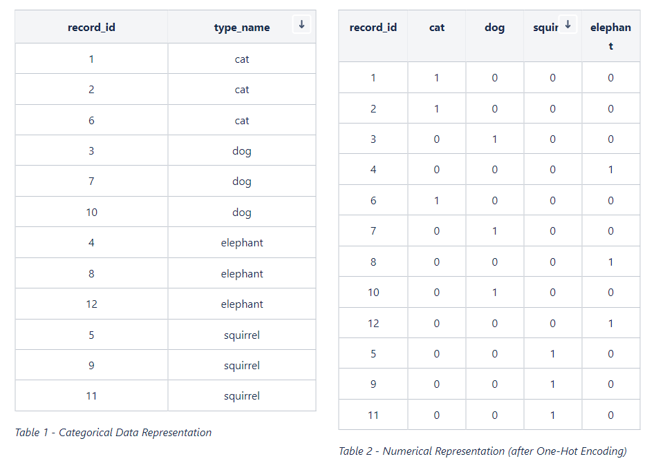
For One-Hot Encoding, we use the function given below.
def convert_to_one_hot(Y, C):
    Y = np.eye(C)[Y.reshape(-1)].T
    return Y
The following code snippet shows how we applied the One-Hot Encoding to data corresponding to the output (Y) from all the available datasets. The code snippet further shows shapes of the numpy arrays after all the previously followed steps.
Y_train = convert_to_one_hot(Y_train_orig, 43).T
Y_val = convert_to_one_hot(Y_val_orig, 43).T
Y_test = convert_to_one_hot(Y_test_orig, 43).T
Y_sv_test = convert_to_one_hot(Y_sv_test_orig, 43).T

print ("Number of Training Examples = " + str(X_train.shape[0]))  // 31367
print ("Number of Validation Examples = " + str(X_val.shape[0]))  // 7842
print ("Number of Test Examples = " + str(X_val.shape[0]))        // 12630
print("X_train shape: " + str(X_train.shape))                     // (31367, 30, 30, 3)
print("Y_train shape: " + str(Y_train.shape))                     // (31367, 43)
print("X_val shape: " + str(X_val.shape))                         // (7842, 30, 30, 3)
print("Y_val shape: " + str(Y_val.shape))                         // (7842, 43)
print("X_test shape: " + str(X_test.shape))                       // (12630, 30, 30, 3)
print("Y_test shape: " + str(Y_test.shape))                       // (12630, 43)
print("X_sv_test shape: " + str(X_sv_test.shape))                 // (32, 30, 30, 3)
print("Y_sv_test shape: " + str(Y_sv_test.shape))                 // (32, 43)
Array to Image
If you are curious, you can always convert an array representation of an image to an image, and see the how it actually looks like. The following code snippets show how you can convert an array back to an image.
Sample image from the Train dataset
# Sample image from the Train dataset # Sample image from Street View Sample
index = 36 index = 24
plt.imshow(X_train[index]) plt.imshow(X_sv_test[index])
print ("y = " + str(np.squeeze(Y_train_orig[index]))) print ("y = " + str(np.squeeze(Y_sv_test_orig[index])))
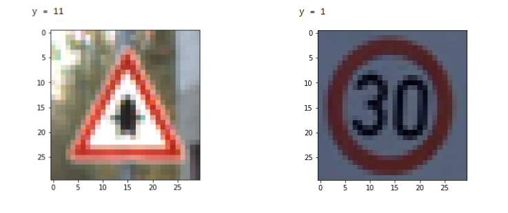
Setting up Commonly Used Functions
We realized that there are tasks that required us to follow almost the same procedure with slight adjustments to the code. From a programming perspective, this is an area where the usage of functions come in handy. We coded up three functions to encapsulate three tasks: 1) Training and Plotting; 2) Plotting; and 3) Evaluation
The following code snippet displays the code blocks used by us. Feel free to make adjustments wherever necessary.
Common Functions
def train_and_plot(model, epochs = 10, batch_size = 64):
    train_dataset = tf.data.Dataset.from_tensor_slices((X_train, Y_train)).batch(batch_size)
    val_dataset = tf.data.Dataset.from_tensor_slices((X_val, Y_val)).batch(batch_size )
    history = model.fit(train_dataset, epochs = epochs, validation_data=val_dataset)
    plot(history)

def plot(history):
    # Plotting the Accuracy variation
    plt.figure(0)
    plt.plot(history.history['accuracy'], label='Training Accuracy')
    plt.plot(history.history['val_accuracy'], label='Validation Accuracy')
    plt.title('Variation of Accuracy')
    plt.xlabel('Epochs')
    plt.ylabel('Accuracy')
    plt.legend()
    plt.show()
    # Plotting the Loss variation
    plt.figure(1)
    plt.plot(history.history['loss'], label='Training Loss')
    plt.plot(history.history['val_loss'], label='Validation Loss')
    plt.title('Loss')
    plt.xlabel('Epochs')
    plt.ylabel('Loss')
    plt.legend()
    plt.show()

def evaluate_validation(model, no_of_images, rows, columns, dataset_type):
    X_ds = None
    Y_ds = None
    Y_orig_ds = None
    result_title = None

    if dataset_type == 'test':
        X_ds = X_test
        Y_ds = Y_test
        Y_orig_ds = Y_test_orig
        result_title = "TEST"
    elif dataset_type == 'val':
        X_ds = X_val
        Y_ds = Y_val
        Y_orig_ds = Y_val_orig
        result_title = "VALIDATION"
    else:
        X_ds = X_sv_test
        Y_ds = Y_sv_test
        Y_orig_ds = Y_sv_test_orig
        result_title = "STREETVIEW TEST"

    eval_result = model.evaluate(X_ds, Y_ds)
    pred = model.predict(X_ds)
    pred_label = [np.argmax(x) for x in pred]

    plt.figure(figsize=(25, 25))
    for i in range(no_of_images):
        plt.subplot(rows, columns, i + 1)
        if (pred_label[i] == Y_orig_ds[i]):
            plt.title(str(pred_label[i]) + " - CORRECT")
        else:
            plt.title(str(pred_label[i]) + " - INCORRECT")
        plt.imshow(X_ds[i])
        plt.axis("off")
    plt.show()

    y_actu = pd.Series(Y_orig_ds, name='Actual')
    y_pred = pd.Series(pred_label, name='Predicted')
    conf_matrix = pd.crosstab(y_actu, y_pred)

    print(conf_matrix)
    accuracy = np.diag(conf_matrix).sum() / conf_matrix.to_numpy().sum()
    print("######################")
    print(result_title + " Accuracy: " + str(round(eval_result[1],4)*100) + "%")
    print("######################")
Model Development - The Iterative Cycle
This will be the longest section of the article as we attempt to explain the thought process behind each tried and tested model. For each model, we will try to be as descriptive as possible and the corresponding results of each model, will also be shown in this section itself (rather than using a different section for Results).
In this section, you will be guided through the process followed by us in implementing and improving the models in an iterative manner. Since this is an iterative procedure, the model accuracy was considered as the single number evaluation metric, and the improvements/modifications are made to models based on the result of the model accuracy obtained by evaluating the validation dataset.
Model 001
The initial model was created to represent the most basic neural network with Input > Dense where we used Adam as the optimizer.
def convolutional_model(input_shape):
    input_img = tf.keras.Input(shape=input_shape)
    F = tf.keras.layers.Flatten()(input_img)
    outputs = tf.keras.layers.Dense(units = 43, activation = 'softmax')(F)
    model = tf.keras.Model(inputs=input_img, outputs=outputs)
    return model

conv_model_v1 = convolutional_model((30, 30, 3))
conv_model_v1.compile(optimizer='adam',
                  loss='categorical_crossentropy',
                  metrics=['accuracy'])
conv_model_v1.summary()
train_and_plot(conv_model_v1)
evaluate_validation(model = conv_model_v1, no_of_images = 32, rows = 7, columns = 7, type = 'val')
Upon training and plotting, the following outcome was obtained. As it turned out, a validation accuracy of 90.16% was achieved. For a basic neural network, this was an excellent result.
Training and Plotting Results - Model 001

Epoch 1/10
491/491 [==============================] - 2s 4ms/step - loss: 2.0973 - accuracy: 0.5373 - val_loss: 1.4628 - val_accuracy: 0.7042
Epoch 2/10
491/491 [==============================] - 2s 3ms/step - loss: 1.2372 - accuracy: 0.7553 - val_loss: 1.0785 - val_accuracy: 0.7844
Epoch 3/10
491/491 [==============================] - 2s 3ms/step - loss: 0.9560 - accuracy: 0.8221 - val_loss: 0.8889 - val_accuracy: 0.8213
Epoch 4/10
491/491 [==============================] - 2s 3ms/step - loss: 0.7964 - accuracy: 0.8552 - val_loss: 0.7673 - val_accuracy: 0.8475
Epoch 5/10
491/491 [==============================] - 2s 3ms/step - loss: 0.6903 - accuracy: 0.8755 - val_loss: 0.6821 - val_accuracy: 0.8671
Epoch 6/10
491/491 [==============================] - 2s 3ms/step - loss: 0.6133 - accuracy: 0.8893 - val_loss: 0.6203 - val_accuracy: 0.8795
Epoch 7/10
491/491 [==============================] - 2s 3ms/step - loss: 0.5540 - accuracy: 0.8992 - val_loss: 0.5724 - val_accuracy: 0.8898
Epoch 8/10
491/491 [==============================] - 2s 3ms/step - loss: 0.5067 - accuracy: 0.9078 - val_loss: 0.5360 - val_accuracy: 0.8949
Epoch 9/10
491/491 [==============================] - 2s 3ms/step - loss: 0.4680 - accuracy: 0.9141 - val_loss: 0.5084 - val_accuracy: 0.8999
Epoch 10/10
491/491 [==============================] - 2s 3ms/step - loss: 0.4354 - accuracy: 0.9195 - val_loss: 0.4859 - val_accuracy: 0.9016
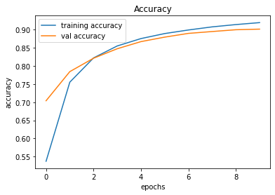
246/246 [==============================] - 0s 2ms/step - loss: 0.4859 - accuracy: 0.9016
######################
VALIDATION Accuracy: 90.16%
######################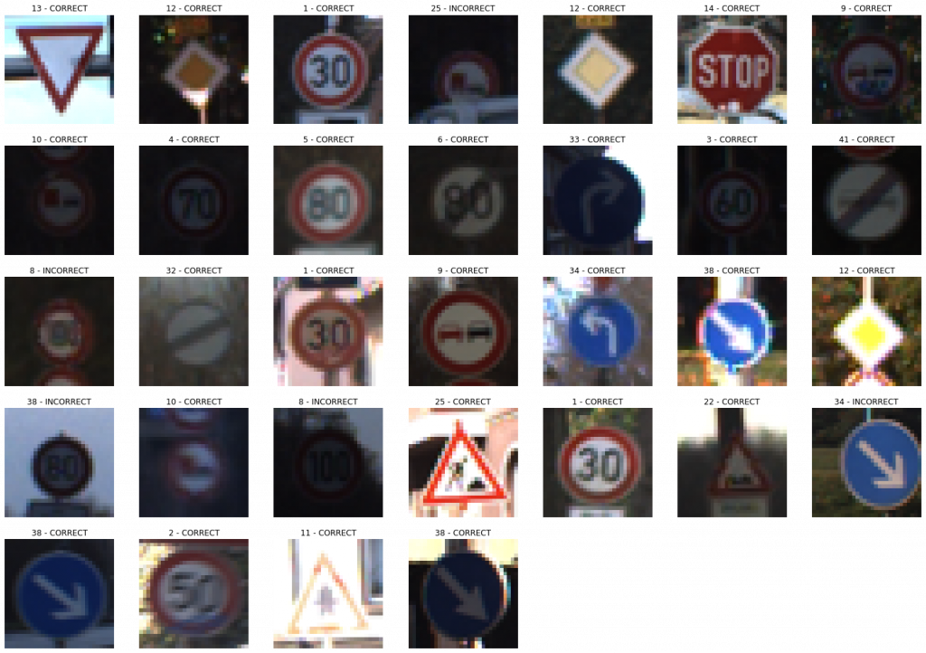
Model 002
In this model, the Model 001 is improved by adding a convolutional layer.
def convolutional_model(input_shape):
    input_img = tf.keras.Input(shape=input_shape)
    Z1 = tf.keras.layers.Conv2D(filters=32, kernel_size= (5, 5), activation = 'relu')(input_img)
    F = tf.keras.layers.Flatten()(Z1)
    outputs = tf.keras.layers.Dense(units = 43, activation = 'softmax')(F)
    model = tf.keras.Model(inputs=input_img, outputs=outputs)
    return model

conv_model_v2 = convolutional_model((30, 30, 3))
conv_model_v2.compile(optimizer='adam',
                  loss='categorical_crossentropy',
                  metrics=['accuracy'])
conv_model_v2.summary()
train_and_plot(conv_model_v2, epochs = 10)
evaluate_validation(model = conv_model_v2, no_of_images = 49, rows = 7, columns = 7, type = 'val')
After training, the validation accuracy was increased by the model up to 97.13%. Can we improve it further?
Validation Accuracy of Model 001 = 90.16%Validation Accuracy of Model 002 = 97.13%
Training and Plotting Results - Model 002

Epoch 1/10
491/491 [==============================] - 14s 29ms/step - loss: 0.8728 - accuracy: 0.7880 - val_loss: 0.3256 - val_accuracy: 0.9299
Epoch 2/10
491/491 [==============================] - 14s 29ms/step - loss: 0.2117 - accuracy: 0.9495 - val_loss: 0.2012 - val_accuracy: 0.9569
Epoch 3/10
491/491 [==============================] - 14s 28ms/step - loss: 0.1183 - accuracy: 0.9723 - val_loss: 0.1655 - val_accuracy: 0.9647
Epoch 4/10
491/491 [==============================] - 14s 29ms/step - loss: 0.0850 - accuracy: 0.9796 - val_loss: 0.1794 - val_accuracy: 0.9588
Epoch 5/10
491/491 [==============================] - 14s 29ms/step - loss: 0.0725 - accuracy: 0.9821 - val_loss: 0.1592 - val_accuracy: 0.9663
Epoch 6/10
491/491 [==============================] - 14s 29ms/step - loss: 0.0491 - accuracy: 0.9869 - val_loss: 0.1543 - val_accuracy: 0.9644
Epoch 7/10
491/491 [==============================] - 15s 30ms/step - loss: 0.0519 - accuracy: 0.9866 - val_loss: 0.1247 - val_accuracy: 0.9748
Epoch 8/10
491/491 [==============================] - 14s 29ms/step - loss: 0.0389 - accuracy: 0.9898 - val_loss: 0.1205 - val_accuracy: 0.9773
Epoch 9/10
491/491 [==============================] - 14s 29ms/step - loss: 0.0301 - accuracy: 0.9928 - val_loss: 0.1227 - val_accuracy: 0.9773
Epoch 10/10
491/491 [==============================] - 15s 30ms/step - loss: 0.0271 - accuracy: 0.9930 - val_loss: 0.1390 - val_accuracy: 0.9713
246/246 [==============================] - 1s 6ms/step - loss: 0.1390 - accuracy: 0.9713
Model 003
This is an attempted improvement from Model 002 by adding a MaxPool2D layer.
def convolutional_model(input_shape):
    input_img = tf.keras.Input(shape=input_shape)
    Z1 = tf.keras.layers.Conv2D(filters=32, kernel_size= (5, 5), activation = 'relu')(input_img)
    P1 = tf.keras.layers.MaxPool2D(pool_size=(2, 2))(Z1)
    F = tf.keras.layers.Flatten()(P1)
    outputs = tf.keras.layers.Dense(units = 43, activation = 'softmax')(F)
    model = tf.keras.Model(inputs=input_img, outputs=outputs)
    return model

conv_model_v3 = convolutional_model((30, 30, 3))
conv_model_v3.compile(optimizer='adam',
                  loss='categorical_crossentropy',
                  metrics=['accuracy'])
conv_model_v3.summary()
train_and_plot(conv_model_v3, epochs = 10)
evaluate_validation(model = conv_model_v3, no_of_images = 49, rows = 7, columns = 7, type = 'val')
The results between Model 002 and Model 003 are similar. However, there's a noticeable difference between the Training Error and Validation Error and this is an indication of overfitting.
Validation Accuracy of Model 002 = 97.13%Validation Accuracy of Model 003 = 97.45%
Training and Plotting Results - Model 003

Epoch 1/10
491/491 [==============================] - 15s 30ms/step - loss: 1.0802 - accuracy: 0.7429 - val_loss: 0.3993 - val_accuracy: 0.9161
Epoch 2/10
491/491 [==============================] - 15s 30ms/step - loss: 0.2667 - accuracy: 0.9440 - val_loss: 0.2223 - val_accuracy: 0.9510
Epoch 3/10
491/491 [==============================] - 15s 31ms/step - loss: 0.1482 - accuracy: 0.9693 - val_loss: 0.1708 - val_accuracy: 0.9610
Epoch 4/10
491/491 [==============================] - 15s 30ms/step - loss: 0.0971 - accuracy: 0.9806 - val_loss: 0.1510 - val_accuracy: 0.9648
Epoch 5/10
491/491 [==============================] - 16s 32ms/step - loss: 0.0702 - accuracy: 0.9862 - val_loss: 0.1266 - val_accuracy: 0.9727
Epoch 6/10
491/491 [==============================] - 15s 32ms/step - loss: 0.0546 - accuracy: 0.9887 - val_loss: 0.1272 - val_accuracy: 0.9709
Epoch 7/10
491/491 [==============================] - 16s 33ms/step - loss: 0.0561 - accuracy: 0.9885 - val_loss: 0.1198 - val_accuracy: 0.9754
Epoch 8/10
491/491 [==============================] - 15s 31ms/step - loss: 0.0422 - accuracy: 0.9911 - val_loss: 0.1137 - val_accuracy: 0.9770
Epoch 9/10
491/491 [==============================] - 15s 31ms/step - loss: 0.0338 - accuracy: 0.9925 - val_loss: 0.1097 - val_accuracy: 0.9762
Epoch 10/10
491/491 [==============================] - 16s 32ms/step - loss: 0.0277 - accuracy: 0.9942 - val_loss: 0.1169 - val_accuracy: 0.9745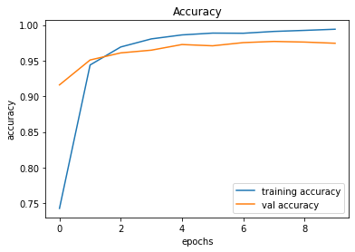
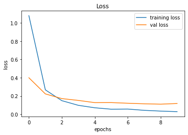
246/246 [==============================] - 1s 6ms/step - loss: 0.1169 - accuracy: 0.9745
Model 004
We will add another Convolutional Layer too see if the results improve to minimize the bias (before focusing on the overfitting problems).
def convolutional_model(input_shape):
    input_img = tf.keras.Input(shape=input_shape)
    Z1 = tf.keras.layers.Conv2D(filters=32, kernel_size= (5, 5), activation = 'relu')(input_img)
    P1 = tf.keras.layers.MaxPool2D(pool_size=(2, 2))(Z1)
    Z2 = tf.keras.layers.Conv2D(filters=64, kernel_size= (5, 5), activation = 'relu')(P1)
    F = tf.keras.layers.Flatten()(Z2)
    outputs = tf.keras.layers.Dense(units = 43, activation = 'softmax')(F)
    model = tf.keras.Model(inputs=input_img, outputs=outputs)
    return model

conv_model_v4 = convolutional_model((30, 30, 3))
conv_model_v4.compile(optimizer='adam',
                  loss='categorical_crossentropy',
                  metrics=['accuracy'])
conv_model_v4.summary()
train_and_plot(conv_model_v4, epochs = 10)
evaluate_validation(model = conv_model_4, no_of_images = 49, rows = 7, columns = 7, type = 'val')
While the validation accuracy improved by approximately 1%, the overfitting problem remains an issue due to the difference between the Training Error and Validation Error.
Validation Accuracy of Model 003 = 97.45%Validation Accuracy of Model 004 = 98.51%
Training and Plotting Results - Model 004

Epoch 1/10
491/491 [==============================] - 26s 53ms/step - loss: 0.8186 - accuracy: 0.7919 - val_loss: 0.2310 - val_accuracy: 0.9498
Epoch 2/10
491/491 [==============================] - 27s 55ms/step - loss: 0.1544 - accuracy: 0.9647 - val_loss: 0.1435 - val_accuracy: 0.9675
Epoch 3/10
491/491 [==============================] - 30s 60ms/step - loss: 0.0759 - accuracy: 0.9824 - val_loss: 0.0957 - val_accuracy: 0.9800
Epoch 4/10
491/491 [==============================] - 29s 59ms/step - loss: 0.0426 - accuracy: 0.9901 - val_loss: 0.0951 - val_accuracy: 0.9796
Epoch 5/10
491/491 [==============================] - 28s 58ms/step - loss: 0.0297 - accuracy: 0.9926 - val_loss: 0.0839 - val_accuracy: 0.9837
Epoch 6/10
491/491 [==============================] - 28s 56ms/step - loss: 0.0223 - accuracy: 0.9942 - val_loss: 0.0870 - val_accuracy: 0.9813
Epoch 7/10
491/491 [==============================] - 27s 55ms/step - loss: 0.0221 - accuracy: 0.9947 - val_loss: 0.0908 - val_accuracy: 0.9816
Epoch 8/10
491/491 [==============================] - 27s 56ms/step - loss: 0.0247 - accuracy: 0.9931 - val_loss: 0.0877 - val_accuracy: 0.9836
Epoch 9/10
491/491 [==============================] - 27s 56ms/step - loss: 0.0110 - accuracy: 0.9973 - val_loss: 0.1071 - val_accuracy: 0.9821
Epoch 10/10
491/491 [==============================] - 28s 57ms/step - loss: 0.0069 - accuracy: 0.9984 - val_loss: 0.0817 - val_accuracy: 0.9851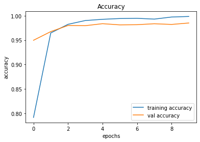
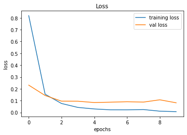
246/246 [==============================] - 2s 8ms/step - loss: 0.0817 - accuracy: 0.9851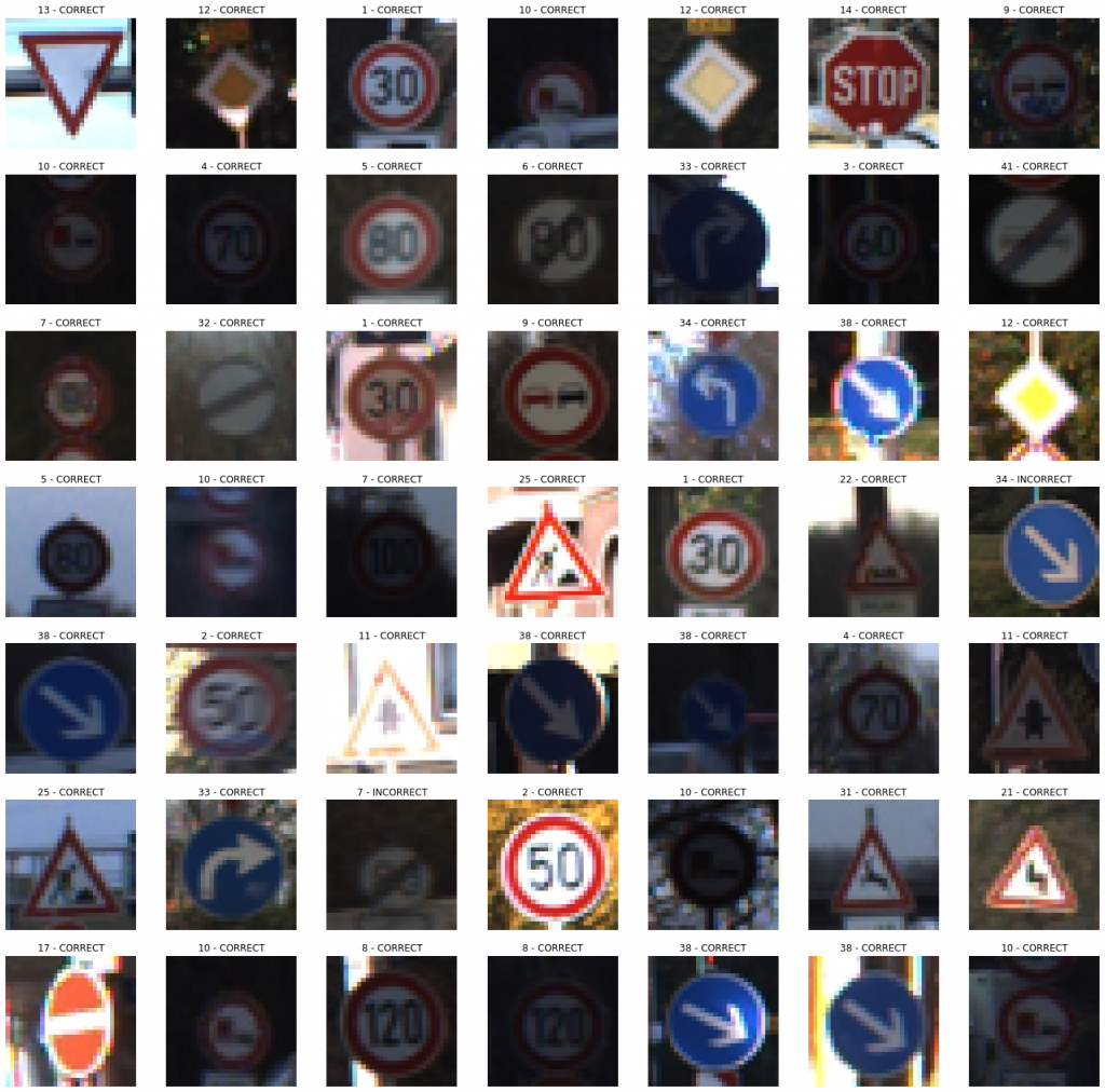
Model 005
We will add another MaxPooling2D Layer before going ahead with the regularization to tackle the overfitting problem.
def convolutional_model(input_shape):
    input_img = tf.keras.Input(shape=input_shape)
    Z1 = tf.keras.layers.Conv2D(filters=32, kernel_size= (5, 5), activation = 'relu')(input_img)
    P1 = tf.keras.layers.MaxPool2D(pool_size=(2, 2))(Z1)
    Z2 = tf.keras.layers.Conv2D(filters=64, kernel_size= (5, 5), activation = 'relu')(P1)
    P2 = tf.keras.layers.MaxPool2D(pool_size=(2, 2))(Z2)
    F = tf.keras.layers.Flatten()(P2)
    outputs = tf.keras.layers.Dense(units = 43, activation = 'softmax')(F)
    model = tf.keras.Model(inputs=input_img, outputs=outputs)
    return model

conv_model_v5 = convolutional_model((30, 30, 3))
conv_model_v5.compile(optimizer='adam',
                  loss='categorical_crossentropy',
                  metrics=['accuracy'])
conv_model_v5.summary()
train_and_plot(conv_model_v8, epochs = 10)
There is a slight improvement in the validation accuracy from 98.51% to 98.83%. However, there is still a slight difference between the training and validation accuracies.
Validation Accuracy of Model 004 = 98.51%Validation Accuracy of Model 005 = 98.83%
Training and Plotting Results - Model 005

Epoch 1/10
491/491 [==============================] - 25s 51ms/step - loss: 1.1546 - accuracy: 0.7134 - val_loss: 0.3212 - val_accuracy: 0.9245
Epoch 2/10
491/491 [==============================] - 25s 50ms/step - loss: 0.2106 - accuracy: 0.9515 - val_loss: 0.1631 - val_accuracy: 0.9611
Epoch 3/10
491/491 [==============================] - 26s 53ms/step - loss: 0.1069 - accuracy: 0.9764 - val_loss: 0.1229 - val_accuracy: 0.9697
Epoch 4/10
491/491 [==============================] - 26s 54ms/step - loss: 0.0641 - accuracy: 0.9858 - val_loss: 0.1016 - val_accuracy: 0.9749
Epoch 5/10
491/491 [==============================] - 27s 54ms/step - loss: 0.0441 - accuracy: 0.9908 - val_loss: 0.0819 - val_accuracy: 0.9815
Epoch 6/10
491/491 [==============================] - 26s 54ms/step - loss: 0.0311 - accuracy: 0.9936 - val_loss: 0.0754 - val_accuracy: 0.9829
Epoch 7/10
491/491 [==============================] - 27s 55ms/step - loss: 0.0274 - accuracy: 0.9935 - val_loss: 0.1225 - val_accuracy: 0.9750
Epoch 8/10
491/491 [==============================] - 26s 53ms/step - loss: 0.0188 - accuracy: 0.9956 - val_loss: 0.0646 - val_accuracy: 0.9846
Epoch 9/10
491/491 [==============================] - 25s 51ms/step - loss: 0.0211 - accuracy: 0.9951 - val_loss: 0.0637 - val_accuracy: 0.9866
Epoch 10/10
491/491 [==============================] - 25s 51ms/step - loss: 0.0170 - accuracy: 0.9960 - val_loss: 0.0621 - val_accuracy: 0.9883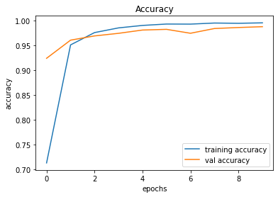
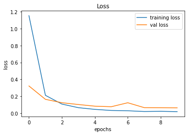
246/246 [==============================] - 2s 8ms/step - loss: 0.0621 - accuracy: 0.9883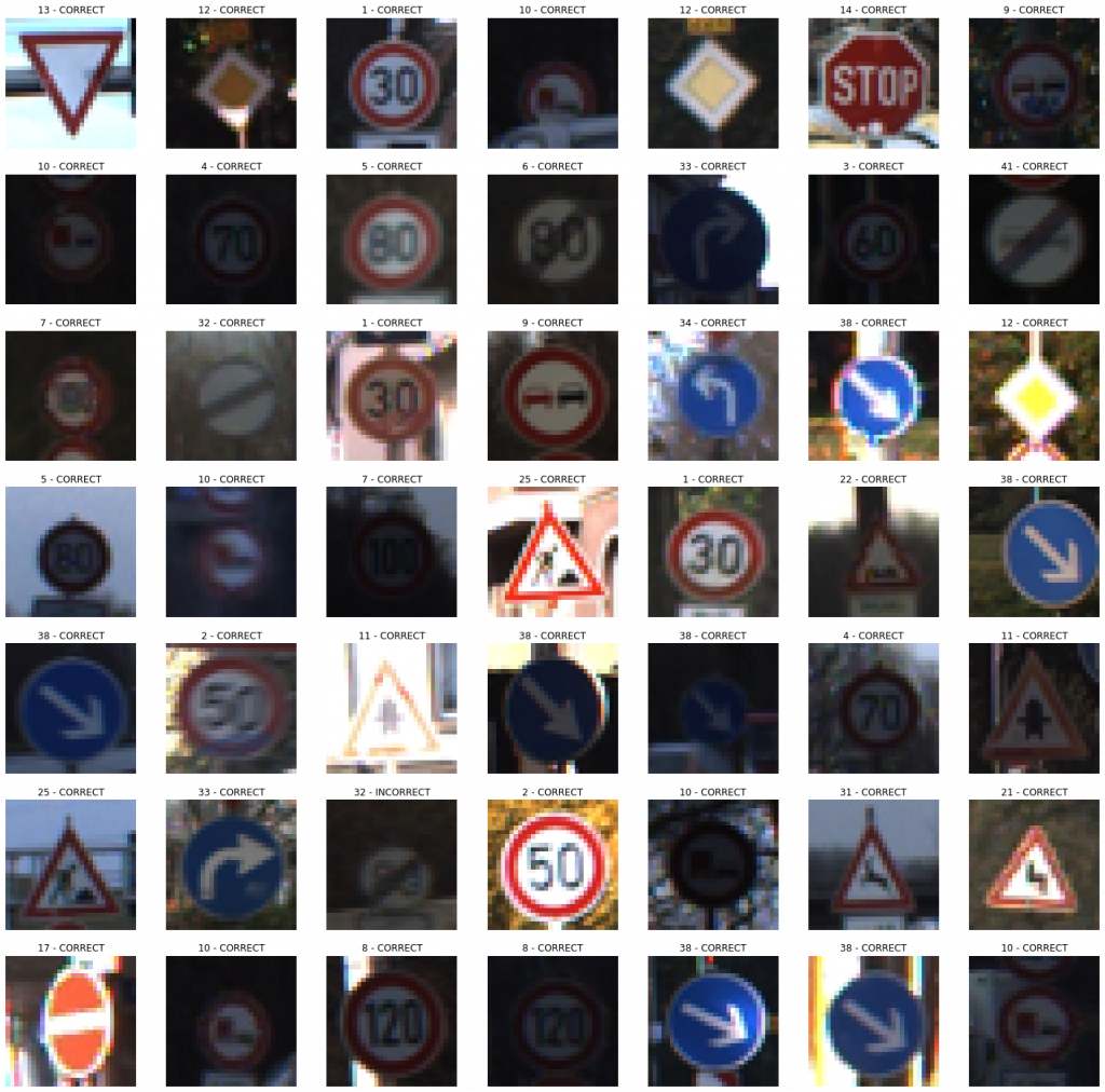
Model 006
Because of the difference between the training and validation accuracies, we are now adding a Dropout layer to address the overfitting problem.
def convolutional_model(input_shape):
    input_img = tf.keras.Input(shape=input_shape)
    Z1 = tf.keras.layers.Conv2D(filters=32, kernel_size= (5, 5), activation = 'relu')(input_img)
    P1 = tf.keras.layers.MaxPool2D(pool_size=(2, 2))(Z1)
    D1 = tf.keras.layers.Dropout(rate = 0.25)(P1)
    Z2 = tf.keras.layers.Conv2D(filters=64, kernel_size= (5, 5), activation = 'relu')(D1)
    P2 = tf.keras.layers.MaxPool2D(pool_size=(2, 2))(Z2)
    F = tf.keras.layers.Flatten()(P2)
    outputs = tf.keras.layers.Dense(units = 43, activation = 'softmax')(F)
    model = tf.keras.Model(inputs=input_img, outputs=outputs)
    return model

conv_model_v6 = convolutional_model((30, 30, 3))
conv_model_v6.compile(optimizer='adam',
                  loss='categorical_crossentropy',
                  metrics=['accuracy'])
conv_model_v6.summary()
train_and_plot(conv_model_v6, epochs = 10)
evaluate_validation(model = conv_model_v6, no_of_images = 49, rows = 7, columns = 7, type = 'val')
The Dropout certainly had an effect in narrowing down the gap between Training Error and Validation Error. However, there is an indication of validation accuracy going down after Epoch 09. In such cases, Early Stopping may come in handy.
Validation Accuracy of Model 005 = 98.83%Validation Accuracy of Model 006 = 98.83%
Training and Plotting Results - Model 006

Epoch 1/10
491/491 [==============================] - 29s 59ms/step - loss: 1.2292 - accuracy: 0.6867 - val_loss: 0.3695 - val_accuracy: 0.9115
Epoch 2/10
491/491 [==============================] - 29s 59ms/step - loss: 0.2606 - accuracy: 0.9351 - val_loss: 0.1708 - val_accuracy: 0.9634
Epoch 3/10
491/491 [==============================] - 30s 62ms/step - loss: 0.1393 - accuracy: 0.9661 - val_loss: 0.1292 - val_accuracy: 0.9686
Epoch 4/10
491/491 [==============================] - 30s 61ms/step - loss: 0.0874 - accuracy: 0.9791 - val_loss: 0.0912 - val_accuracy: 0.9802
Epoch 5/10
491/491 [==============================] - 29s 59ms/step - loss: 0.0680 - accuracy: 0.9835 - val_loss: 0.0797 - val_accuracy: 0.9815
Epoch 6/10
491/491 [==============================] - 29s 59ms/step - loss: 0.0496 - accuracy: 0.9882 - val_loss: 0.0736 - val_accuracy: 0.9847
Epoch 7/10
491/491 [==============================] - 30s 60ms/step - loss: 0.0411 - accuracy: 0.9896 - val_loss: 0.0669 - val_accuracy: 0.9846
Epoch 8/10
491/491 [==============================] - 29s 60ms/step - loss: 0.0362 - accuracy: 0.9899 - val_loss: 0.0481 - val_accuracy: 0.9894
Epoch 9/10
491/491 [==============================] - 30s 60ms/step - loss: 0.0285 - accuracy: 0.9928 - val_loss: 0.0496 - val_accuracy: 0.9888
Epoch 10/10
491/491 [==============================] - 30s 61ms/step - loss: 0.0259 - accuracy: 0.9936 - val_loss: 0.0557 - val_accuracy: 0.9883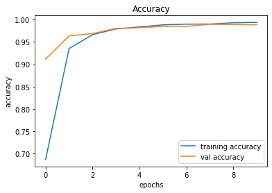
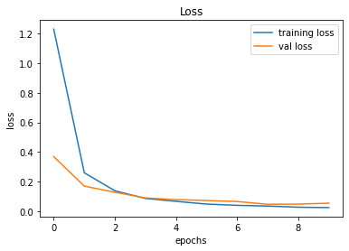
246/246 [==============================] - 2s 8ms/step - loss: 0.0557 - accuracy: 0.9883
Model 007
We will add another Dropout layer to see if we can further fine-tune the model and then let's proceed with Early Stopping if necessary.
# Model 007

def convolutional_model(input_shape):
    input_img = tf.keras.Input(shape=input_shape)
    Z1 = tf.keras.layers.Conv2D(filters=32, kernel_size= (5, 5), activation = 'relu')(input_img)
    P1 = tf.keras.layers.MaxPool2D(pool_size=(2, 2))(Z1)
    D1 = tf.keras.layers.Dropout(rate = 0.25)(P1)
    Z2 = tf.keras.layers.Conv2D(filters=64, kernel_size= (5, 5), activation = 'relu')(D1)
    P2 = tf.keras.layers.MaxPool2D(pool_size=(2, 2))(Z2)
    D2 = tf.keras.layers.Dropout(rate = 0.25)(P2)
    F = tf.keras.layers.Flatten()(D2)
    outputs = tf.keras.layers.Dense(units = 43, activation = 'softmax')(F)
    model = tf.keras.Model(inputs=input_img, outputs=outputs)
    return model

conv_model_v7 = convolutional_model((30, 30, 3))
conv_model_v7.compile(optimizer='adam',
                  loss='categorical_crossentropy',
                  metrics=['accuracy'])
conv_model_v7.summary()
train_and_plot(conv_model_v7, epochs = 10)
evaluate_validation(model = conv_model_v7, no_of_images = 49, rows = 7, columns = 7, type = 'val')
The validation accuracy slightly improved from 98.83% to 99.22%.
Validation Accuracy of Model 006 = 98.83%Validation Accuracy of Model 007 = 99.22%
Training and Plotting Results - Model 007

Epoch 1/10
491/491 [==============================] - 30s 61ms/step - loss: 1.3423 - accuracy: 0.6474 - val_loss: 0.3653 - val_accuracy: 0.9217
Epoch 2/10
491/491 [==============================] - 30s 62ms/step - loss: 0.3166 - accuracy: 0.9155 - val_loss: 0.1653 - val_accuracy: 0.9675
Epoch 3/10
491/491 [==============================] - 31s 64ms/step - loss: 0.1760 - accuracy: 0.9539 - val_loss: 0.1124 - val_accuracy: 0.9784
Epoch 4/10
491/491 [==============================] - 36s 74ms/step - loss: 0.1198 - accuracy: 0.9687 - val_loss: 0.0857 - val_accuracy: 0.9844
Epoch 5/10
491/491 [==============================] - 39s 80ms/step - loss: 0.0861 - accuracy: 0.9769 - val_loss: 0.0709 - val_accuracy: 0.9837
Epoch 6/10
491/491 [==============================] - 32s 66ms/step - loss: 0.0710 - accuracy: 0.9808 - val_loss: 0.0517 - val_accuracy: 0.9892
Epoch 7/10
491/491 [==============================] - 41s 84ms/step - loss: 0.0621 - accuracy: 0.9830 - val_loss: 0.0535 - val_accuracy: 0.9895
Epoch 8/10
491/491 [==============================] - 34s 68ms/step - loss: 0.0486 - accuracy: 0.9868 - val_loss: 0.0422 - val_accuracy: 0.9922
Epoch 9/10
491/491 [==============================] - 30s 61ms/step - loss: 0.0424 - accuracy: 0.9881 - val_loss: 0.0458 - val_accuracy: 0.9903
Epoch 10/10
491/491 [==============================] - 30s 62ms/step - loss: 0.0416 - accuracy: 0.9881 - val_loss: 0.0387 - val_accuracy: 0.9922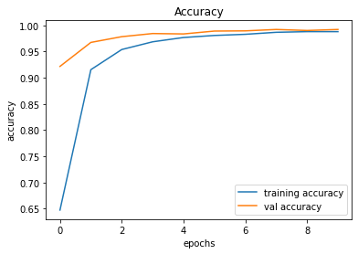
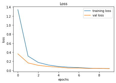
246/246 [==============================] - 2s 8ms/step - loss: 0.0387 - accuracy: 0.9922
Model 008
Adding more layers make the network deeper and having a bigger network almost always helps in minimizing the bias, and for increasing the accuracy. Therefore, we will add another Convolutional Layer to see if we can further increase the Validation Accuracy. On the other hand, the validation accuracy surpassed the training accuracy, and this happens due to the effect of Dropout.
def convolutional_model(input_shape):
    input_img = tf.keras.Input(shape=input_shape)
    Z1 = tf.keras.layers.Conv2D(filters=32, kernel_size= (5, 5), activation = 'relu')(input_img)
    P1 = tf.keras.layers.MaxPool2D(pool_size=(2, 2))(Z1)
    D1 = tf.keras.layers.Dropout(rate = 0.25)(P1)
    Z2 = tf.keras.layers.Conv2D(filters=64, kernel_size= (5, 5), activation = 'relu')(D1)
    P2 = tf.keras.layers.MaxPool2D(pool_size=(2, 2))(Z2)
    D2 = tf.keras.layers.Dropout(rate = 0.25)(P2)
    Z3 = tf.keras.layers.Conv2D(filters=256, kernel_size= (3, 3), activation = 'relu')(D2)
    F = tf.keras.layers.Flatten()(Z3)
    outputs = tf.keras.layers.Dense(units = 43, activation = 'softmax')(F)
    model = tf.keras.Model(inputs=input_img, outputs=outputs)
    return model

conv_model_v8 = convolutional_model((30, 30, 3))
conv_model_v8.compile(optimizer='adam',
                  loss='categorical_crossentropy',
                  metrics=['accuracy'])
conv_model_v8.summary()
train_and_plot(conv_model_v8, epochs = 10)
evaluate_validation(model = conv_model_v8, no_of_images = 49, rows = 7, columns = 7, type = 'val')
The validation accuracy slightly improved from 99.22% to 99.34%.
Validation Accuracy of Model 007 = 98.22%Validation Accuracy of Model 008 = 99.34%
Training and Plotting Results - Model 008
Epoch 1/10
491/491 [==============================] - 31s 63ms/step - loss: 1.1019 - accuracy: 0.6988 - val_loss: 0.2339 - val_accuracy: 0.9439
Epoch 2/10
491/491 [==============================] - 32s 65ms/step - loss: 0.2157 - accuracy: 0.9404 - val_loss: 0.1071 - val_accuracy: 0.9740
Epoch 3/10
491/491 [==============================] - 35s 72ms/step - loss: 0.1245 - accuracy: 0.9656 - val_loss: 0.0783 - val_accuracy: 0.9830
Epoch 4/10
491/491 [==============================] - 33s 67ms/step - loss: 0.0837 - accuracy: 0.9761 - val_loss: 0.0574 - val_accuracy: 0.9892
Epoch 5/10
491/491 [==============================] - 34s 70ms/step - loss: 0.0669 - accuracy: 0.9806 - val_loss: 0.0595 - val_accuracy: 0.9884
Epoch 6/10
491/491 [==============================] - 33s 68ms/step - loss: 0.0540 - accuracy: 0.9848 - val_loss: 0.0446 - val_accuracy: 0.9926
Epoch 7/10
491/491 [==============================] - 35s 71ms/step - loss: 0.0424 - accuracy: 0.9877 - val_loss: 0.0486 - val_accuracy: 0.9899
Epoch 8/10
491/491 [==============================] - 33s 68ms/step - loss: 0.0447 - accuracy: 0.9868 - val_loss: 0.0429 - val_accuracy: 0.9911
Epoch 9/10
491/491 [==============================] - 36s 73ms/step - loss: 0.0405 - accuracy: 0.9879 - val_loss: 0.0373 - val_accuracy: 0.9930
Epoch 10/10
491/491 [==============================] - 38s 78ms/step - loss: 0.0393 - accuracy: 0.9881 - val_loss: 0.0392 - val_accuracy: 0.9934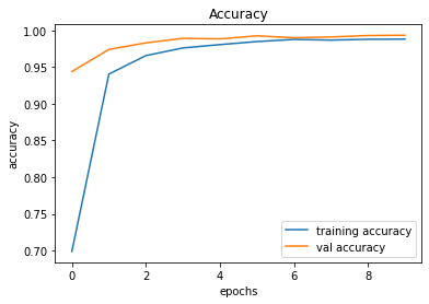
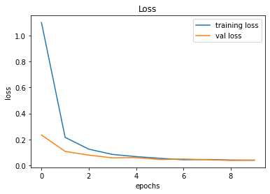
246/246 [==============================] - 2s 10ms/step - loss: 0.0392 - accuracy: 0.9934
Model 009
We further add another MaxPool2D layer, followed by a Dropout layer.
def convolutional_model(input_shape):
    input_img = tf.keras.Input(shape=input_shape)
    Z1 = tf.keras.layers.Conv2D(filters=32, kernel_size= (5, 5), activation = 'relu')(input_img)
    P1 = tf.keras.layers.MaxPool2D(pool_size=(2, 2))(Z1)
    D1 = tf.keras.layers.Dropout(rate = 0.25)(P1)
    Z2 = tf.keras.layers.Conv2D(filters=64, kernel_size= (5, 5), activation = 'relu')(D1)
    P2 = tf.keras.layers.MaxPool2D(pool_size=(2, 2))(Z2)
    D2 = tf.keras.layers.Dropout(rate = 0.25)(P2)
    Z3 = tf.keras.layers.Conv2D(filters=256, kernel_size= (3, 3), activation = 'relu')(D2)
    P3 = tf.keras.layers.MaxPool2D(pool_size=(2, 2))(Z3)
    D3 = tf.keras.layers.Dropout(rate = 0.25)(P3)
    F = tf.keras.layers.Flatten()(D3)
    outputs = tf.keras.layers.Dense(units = 43, activation = 'softmax')(F)
    model = tf.keras.Model(inputs=input_img, outputs=outputs)
    return model

conv_model_v9 = convolutional_model((30, 30, 3))
conv_model_v9.compile(optimizer='adam',
                  loss='categorical_crossentropy',
                  metrics=['accuracy'])
conv_model_v9.summary()
train_and_plot(conv_model_v9, epochs = 10)
evaluate_validation(model = conv_model_v9, no_of_images = 49, rows = 7, columns = 7, type = 'val')
The validation accuracy slightly improved from 99.34% to 99.36%.
Validation Accuracy of Model 008 = 98.34%Validation Accuracy of Model 009 = 99.36%Training and Plotting Result - Model 009
Training and Plotting Results - Model 009

Epoch 1/10
491/491 [==============================] - 32s 64ms/step - loss: 1.8729 - accuracy: 0.4747 - val_loss: 0.4384 - val_accuracy: 0.8979
Epoch 2/10
491/491 [==============================] - 33s 66ms/step - loss: 0.4269 - accuracy: 0.8749 - val_loss: 0.1343 - val_accuracy: 0.9718
Epoch 3/10
491/491 [==============================] - 34s 69ms/step - loss: 0.2201 - accuracy: 0.9376 - val_loss: 0.0722 - val_accuracy: 0.9852
Epoch 4/10
491/491 [==============================] - 34s 69ms/step - loss: 0.1456 - accuracy: 0.9567 - val_loss: 0.0498 - val_accuracy: 0.9895
Epoch 5/10
491/491 [==============================] - 34s 69ms/step - loss: 0.1102 - accuracy: 0.9676 - val_loss: 0.0382 - val_accuracy: 0.9926
Epoch 6/10
491/491 [==============================] - 34s 70ms/step - loss: 0.0923 - accuracy: 0.9729 - val_loss: 0.0380 - val_accuracy: 0.9932
Epoch 7/10
491/491 [==============================] - 34s 69ms/step - loss: 0.0773 - accuracy: 0.9774 - val_loss: 0.0426 - val_accuracy: 0.9902
Epoch 8/10
491/491 [==============================] - 33s 67ms/step - loss: 0.0692 - accuracy: 0.9800 - val_loss: 0.0265 - val_accuracy: 0.9943
Epoch 9/10
491/491 [==============================] - 32s 66ms/step - loss: 0.0570 - accuracy: 0.9839 - val_loss: 0.0249 - val_accuracy: 0.9939
Epoch 10/10
491/491 [==============================] - 32s 65ms/step - loss: 0.0630 - accuracy: 0.9807 - val_loss: 0.0290 - val_accuracy: 0.9936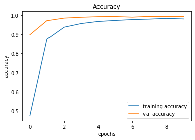
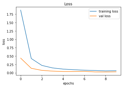
Model 010
Now, we will add a Fully Connected Layer to see if it improves the overall performance (and minimize the bias).
def convolutional_model(input_shape):
    input_img = tf.keras.Input(shape=input_shape)
    Z1 = tf.keras.layers.Conv2D(filters=32, kernel_size= (5, 5), activation = 'relu')(input_img)
    P1 = tf.keras.layers.MaxPool2D(pool_size=(2, 2))(Z1)
    D1 = tf.keras.layers.Dropout(rate = 0.25)(P1)
    Z2 = tf.keras.layers.Conv2D(filters=64, kernel_size= (5, 5), activation = 'relu')(D1)
    P2 = tf.keras.layers.MaxPool2D(pool_size=(2, 2))(Z2)
    D2 = tf.keras.layers.Dropout(rate = 0.25)(P2)
    Z3 = tf.keras.layers.Conv2D(filters=256, kernel_size= (3, 3), activation = 'relu')(D2)
    P3 = tf.keras.layers.MaxPool2D(pool_size=(2, 2))(Z3)
    D3 = tf.keras.layers.Dropout(rate = 0.25)(P3)
    F = tf.keras.layers.Flatten()(D3)
    FC1 = tf.keras.layers.Dense(units = 256, activation = 'relu')(F)
    outputs = tf.keras.layers.Dense(units = 43, activation = 'softmax')(FC1)
    model = tf.keras.Model(inputs=input_img, outputs=outputs)
    return model

conv_model_v10 = convolutional_model((30, 30, 3))
conv_model_v10.compile(optimizer='adam',
                  loss='categorical_crossentropy',
                  metrics=['accuracy'])
conv_model_v10.summary()
train_and_plot(conv_model_v10, epochs = 10)
Validation Accuracy of Model 009 = 98.36%Validation Accuracy of Model 010 = 99.38%
Training and Plotting Results - Model 010

Epoch 1/10
491/491 [==============================] - 31s 63ms/step - loss: 2.0385 - accuracy: 0.4115 - val_loss: 0.4938 - val_accuracy: 0.8601
Epoch 2/10
491/491 [==============================] - 31s 63ms/step - loss: 0.4200 - accuracy: 0.8677 - val_loss: 0.1395 - val_accuracy: 0.9675
Epoch 3/10
491/491 [==============================] - 32s 66ms/step - loss: 0.2112 - accuracy: 0.9377 - val_loss: 0.0846 - val_accuracy: 0.9793
Epoch 4/10
491/491 [==============================] - 32s 65ms/step - loss: 0.1538 - accuracy: 0.9545 - val_loss: 0.0630 - val_accuracy: 0.9856
Epoch 5/10
491/491 [==============================] - 32s 65ms/step - loss: 0.1147 - accuracy: 0.9645 - val_loss: 0.0494 - val_accuracy: 0.9878
Epoch 6/10
491/491 [==============================] - 32s 65ms/step - loss: 0.0984 - accuracy: 0.9698 - val_loss: 0.0545 - val_accuracy: 0.9858
Epoch 7/10
491/491 [==============================] - 32s 66ms/step - loss: 0.0881 - accuracy: 0.9729 - val_loss: 0.0326 - val_accuracy: 0.9918
Epoch 8/10
491/491 [==============================] - 32s 65ms/step - loss: 0.0778 - accuracy: 0.9764 - val_loss: 0.0275 - val_accuracy: 0.9935
Epoch 9/10
491/491 [==============================] - 32s 65ms/step - loss: 0.0679 - accuracy: 0.9787 - val_loss: 0.0291 - val_accuracy: 0.9920
Epoch 10/10
491/491 [==============================] - 32s 66ms/step - loss: 0.0736 - accuracy: 0.9782 - val_loss: 0.0226 - val_accuracy: 0.9938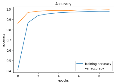
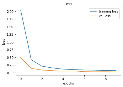
246/246 [==============================] - 2s 9ms/step - loss: 0.0226 - accuracy: 0.9938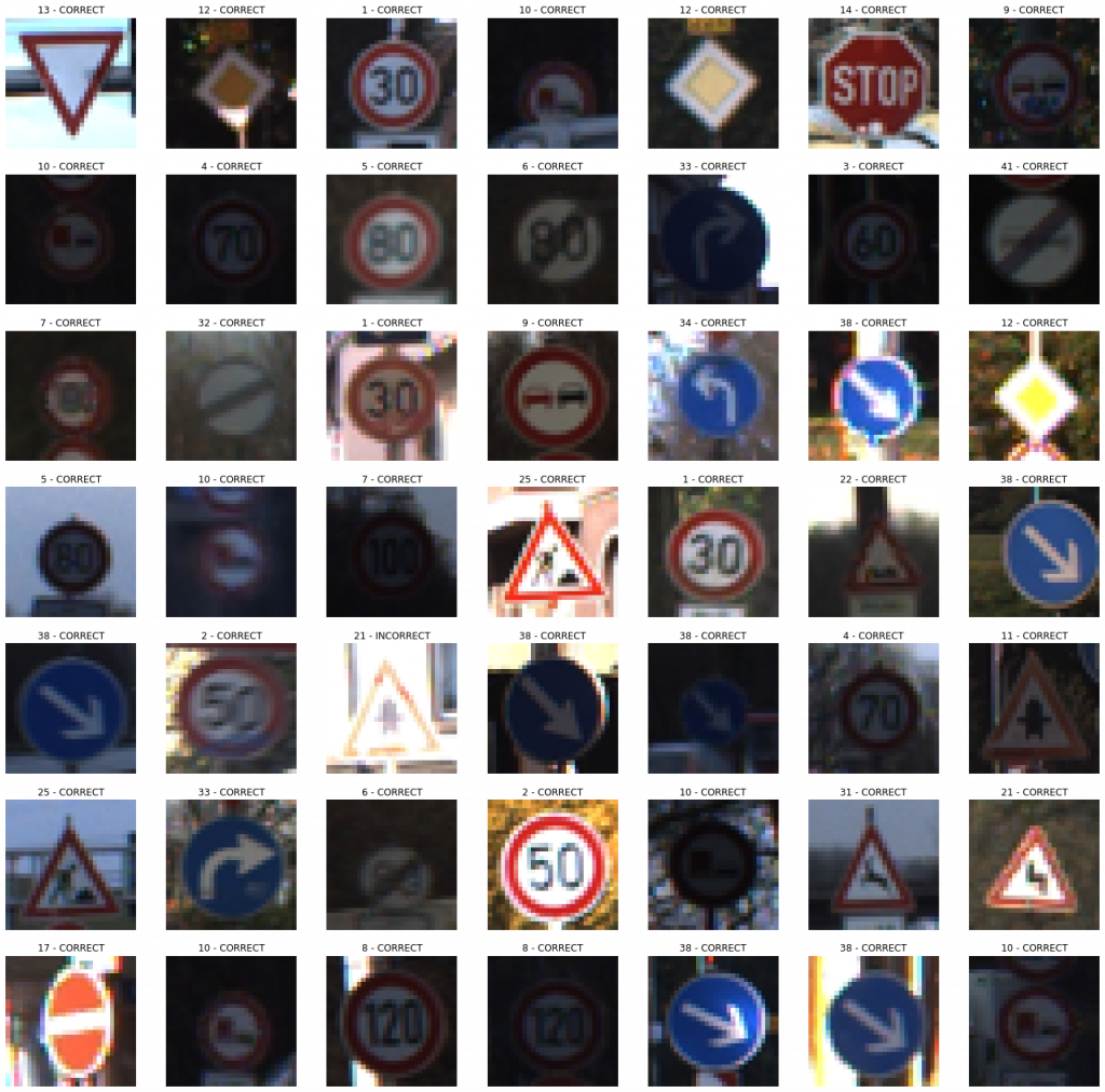
Model 011
While it may not have a considerable effect, it is worth a try to add a regularizer to the Fully Connected Layer.
def convolutional_model(input_shape):
    input_img = tf.keras.Input(shape=input_shape)
    Z1 = tf.keras.layers.Conv2D(filters=32, kernel_size= (5, 5), activation = 'relu')(input_img)
    P1 = tf.keras.layers.MaxPool2D(pool_size=(2, 2))(Z1)
    D1 = tf.keras.layers.Dropout(rate = 0.25)(P1)
    Z2 = tf.keras.layers.Conv2D(filters=64, kernel_size= (5, 5), activation = 'relu')(D1)
    P2 = tf.keras.layers.MaxPool2D(pool_size=(2, 2))(Z2)
    D2 = tf.keras.layers.Dropout(rate = 0.25)(P2)
    Z3 = tf.keras.layers.Conv2D(filters=256, kernel_size= (3, 3), activation = 'relu')(D2)
    P3 = tf.keras.layers.MaxPool2D(pool_size=(2, 2))(Z3)
    D3 = tf.keras.layers.Dropout(rate = 0.25)(P3)
    F = tf.keras.layers.Flatten()(D3)
    FC1 = tf.keras.layers.Dense(units = 256, activation = 'relu', kernel_regularizer=regularizers.l2(0.0001))(F)
    outputs = tf.keras.layers.Dense(units = 43, activation = 'softmax')(FC1)
    model = tf.keras.Model(inputs=input_img, outputs=outputs)
    return model

conv_model_v11 = convolutional_model((30, 30, 3))
conv_model_v11.compile(optimizer='adam',
                  loss='categorical_crossentropy',
                  metrics=['accuracy'])
conv_model_v11.summary()
train_and_plot(conv_model_v11, epochs = 10)
evaluate_validation(model = conv_model_v11, no_of_images = 49, rows = 7, columns = 7, type = 'val')
Validation Accuracy of Model 010 = 99.38%Validation Accuracy of Model 011 = 99.44%
Epoch 1/10
491/491 [==============================] - 32s 66ms/step - loss: 1.9605 - accuracy: 0.4357 - val_loss: 0.5152 - val_accuracy: 0.8624
Epoch 2/10
491/491 [==============================] - 34s 69ms/step - loss: 0.4549 - accuracy: 0.8630 - val_loss: 0.1577 - val_accuracy: 0.9679
Epoch 3/10
491/491 [==============================] - 33s 67ms/step - loss: 0.2494 - accuracy: 0.9301 - val_loss: 0.1195 - val_accuracy: 0.9779
Epoch 4/10
491/491 [==============================] - 32s 66ms/step - loss: 0.1742 - accuracy: 0.9527 - val_loss: 0.0850 - val_accuracy: 0.9860
Epoch 5/10
491/491 [==============================] - 32s 66ms/step - loss: 0.1446 - accuracy: 0.9633 - val_loss: 0.0758 - val_accuracy: 0.9889
Epoch 6/10
491/491 [==============================] - 33s 66ms/step - loss: 0.1236 - accuracy: 0.9696 - val_loss: 0.0676 - val_accuracy: 0.9908
Epoch 7/10
491/491 [==============================] - 33s 67ms/step - loss: 0.1121 - accuracy: 0.9726 - val_loss: 0.0618 - val_accuracy: 0.9918
Epoch 8/10
491/491 [==============================] - 34s 68ms/step - loss: 0.1026 - accuracy: 0.9765 - val_loss: 0.0585 - val_accuracy: 0.9920
Epoch 9/10
491/491 [==============================] - 32s 66ms/step - loss: 0.0965 - accuracy: 0.9778 - val_loss: 0.0539 - val_accuracy: 0.9926
Epoch 10/10
491/491 [==============================] - 33s 66ms/step - loss: 0.0914 - accuracy: 0.9789 - val_loss: 0.0495 - val_accuracy: 0.9944
246/246 [==============================] - 2s 10ms/step - loss: 0.0495 - accuracy: 0.9944
Since we have achieved an acceptable accuracy, let us try to train longer by increasing the number of epochs. While training longer does not always help, it never hurts to try training longer.
train_and_plot(conv_model_v11, epochs = 20)Validation Accuracy of Model 011 (with 10 epochs) = 99.44%Validation Accuracy of Model 011 (with 20 epochs) = 99.53%
Epoch 1/20
491/491 [==============================] - 30s 62ms/step - loss: 0.0867 - accuracy: 0.9806 - val_loss: 0.0511 - val_accuracy: 0.9939
Epoch 2/20
491/491 [==============================] - 32s 64ms/step - loss: 0.0804 - accuracy: 0.9834 - val_loss: 0.0518 - val_accuracy: 0.9938
Epoch 3/20
491/491 [==============================] - 34s 69ms/step - loss: 0.0764 - accuracy: 0.9835 - val_loss: 0.0454 - val_accuracy: 0.9948
Epoch 4/20
491/491 [==============================] - 32s 65ms/step - loss: 0.0710 - accuracy: 0.9849 - val_loss: 0.0459 - val_accuracy: 0.9943
Epoch 5/20
491/491 [==============================] - 31s 64ms/step - loss: 0.0719 - accuracy: 0.9844 - val_loss: 0.0494 - val_accuracy: 0.9927
Epoch 6/20
491/491 [==============================] - 31s 64ms/step - loss: 0.0745 - accuracy: 0.9837 - val_loss: 0.0491 - val_accuracy: 0.9941
Epoch 7/20
491/491 [==============================] - 32s 65ms/step - loss: 0.0703 - accuracy: 0.9855 - val_loss: 0.0499 - val_accuracy: 0.9939
Epoch 8/20
491/491 [==============================] - 32s 65ms/step - loss: 0.0694 - accuracy: 0.9853 - val_loss: 0.0545 - val_accuracy: 0.9926
Epoch 9/20
491/491 [==============================] - 33s 67ms/step - loss: 0.0659 - accuracy: 0.9865 - val_loss: 0.0463 - val_accuracy: 0.9952
Epoch 10/20
491/491 [==============================] - 33s 67ms/step - loss: 0.0639 - accuracy: 0.9875 - val_loss: 0.0423 - val_accuracy: 0.9952
Epoch 11/20
491/491 [==============================] - 36s 72ms/step - loss: 0.0603 - accuracy: 0.9873 - val_loss: 0.0386 - val_accuracy: 0.9954
Epoch 12/20
491/491 [==============================] - 32s 66ms/step - loss: 0.0610 - accuracy: 0.9871 - val_loss: 0.0460 - val_accuracy: 0.9935
Epoch 13/20
491/491 [==============================] - 30s 61ms/step - loss: 0.0553 - accuracy: 0.9898 - val_loss: 0.0402 - val_accuracy: 0.9963
Epoch 14/20
491/491 [==============================] - 34s 69ms/step - loss: 0.0625 - accuracy: 0.9869 - val_loss: 0.0393 - val_accuracy: 0.9960
Epoch 15/20
491/491 [==============================] - 40s 81ms/step - loss: 0.0584 - accuracy: 0.9877 - val_loss: 0.0427 - val_accuracy: 0.9957
Epoch 16/20
491/491 [==============================] - 42s 86ms/step - loss: 0.0580 - accuracy: 0.9881 - val_loss: 0.0435 - val_accuracy: 0.9955
Epoch 17/20
491/491 [==============================] - 37s 76ms/step - loss: 0.0532 - accuracy: 0.9900 - val_loss: 0.0431 - val_accuracy: 0.9952
Epoch 18/20
491/491 [==============================] - 35s 71ms/step - loss: 0.0570 - accuracy: 0.9889 - val_loss: 0.0363 - val_accuracy: 0.9959
Epoch 19/20
491/491 [==============================] - 34s 69ms/step - loss: 0.0566 - accuracy: 0.9889 - val_loss: 0.0348 - val_accuracy: 0.9969
Epoch 20/20
491/491 [==============================] - 34s 70ms/step - loss: 0.0517 - accuracy: 0.9896 - val_loss: 0.0423 - val_accuracy: 0.9953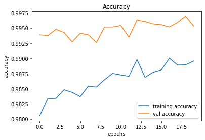
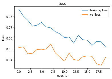
246/246 [==============================] - 2s 8ms/step - loss: 0.0423 - accuracy: 0.9953
We will consider this as the final model because we have been able to achieve a validation accuracy of over 99.50%. The following code snippet should assist us in saving the final model in Hierarchical Data Format version 5 (HDF5).
conv_model_v11.save("gtsrb_v11.h5")Summary
The table given below, summarizes the results of the models that we implemented.
The Test Drive
| Model | Accuracy |
| Model 001 | 90.16% |
| Model 002 | 97.13% |
| Model 003 | 97.45% |
| Model 004 | 98.51% |
| Model 005 | 98.83% |
| Model 006 | 98.83% |
| Model 007 | 99.22% |
| Model 008 | 99.34% |
| Model 009 | 99.36% |
| Model 010 | 99.38% |
| Model 011 | 99.53% |
This section is used for explaining the results and implications from the Test phase. The emphasis will be placed for detailing out the specific outcomes from both the Test Dataset and the Custom Street View Test Dataset.
In the previous section, we finally chose Model 011 as the final model because of its high validation accuracy. In this section, we will be applying Model 011 on two completely unseen (left out) Test datasets to see its robustness on a production run. Therefore, the model will be applied first to the Test dataset that came from the original dataset.
evaluate_validation(model = conv_model_v11, no_of_images = 49, rows = 7, columns = 7, type = 'test')395/395 [==============================] - 3s 9ms/step - loss: 0.2013 - accuracy: 0.96371
######################
TEST Accuracy: 96.37%
######################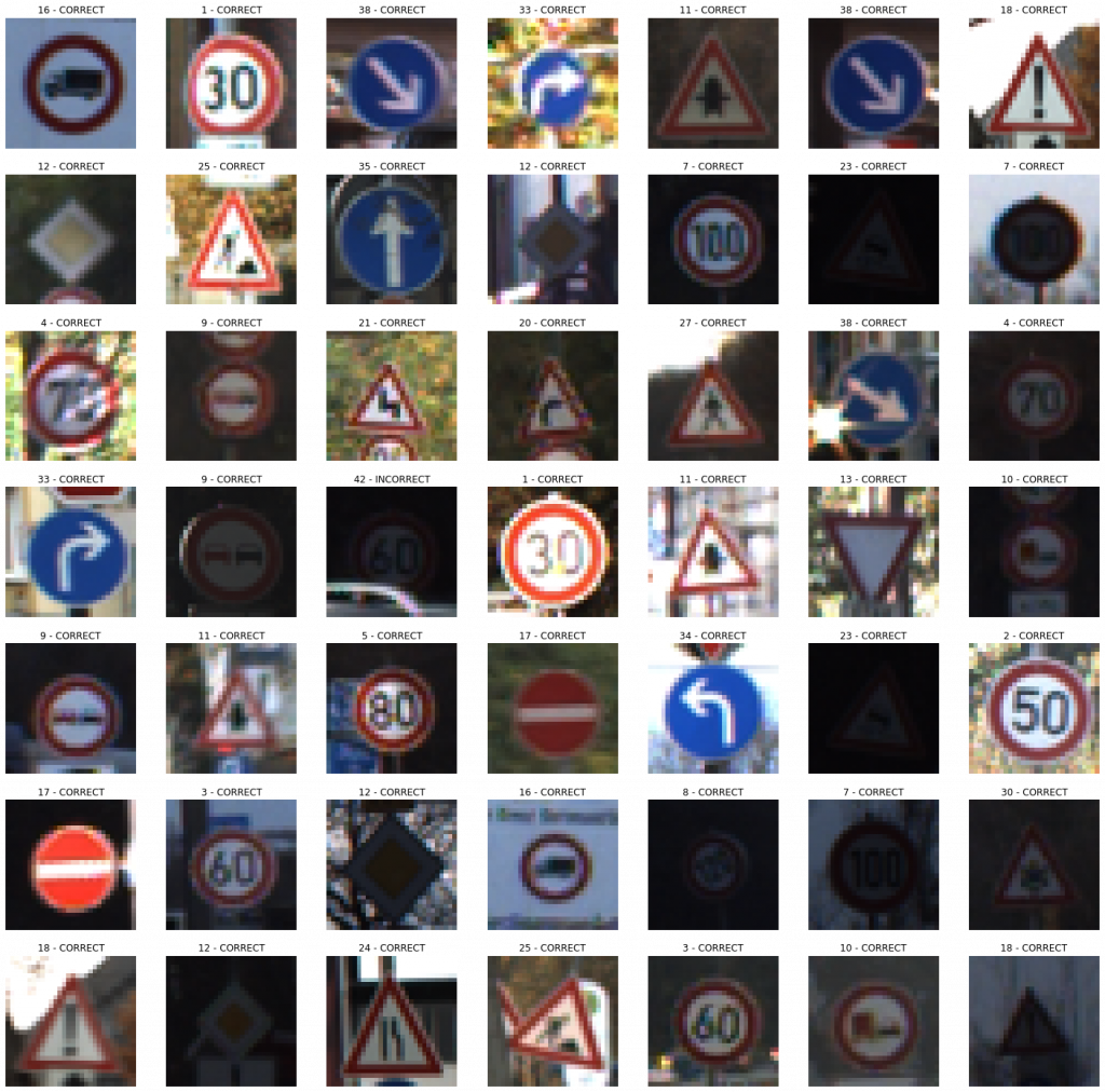
Voila! The model managed to achieve an accuracy of 96.37% on the completely unseen dataset. Let us see how it performs on the images captured from Google Street View.
evaluate_validation(model = conv_model_v11, no_of_images = 32, rows = 6, columns = 6, type = 'sv')1/1 [==============================] - 0s 1ms/step - loss: 0.0781 - accuracy: 0.9688
######################
STREETVIEW TEST Accuracy: 96.88%
######################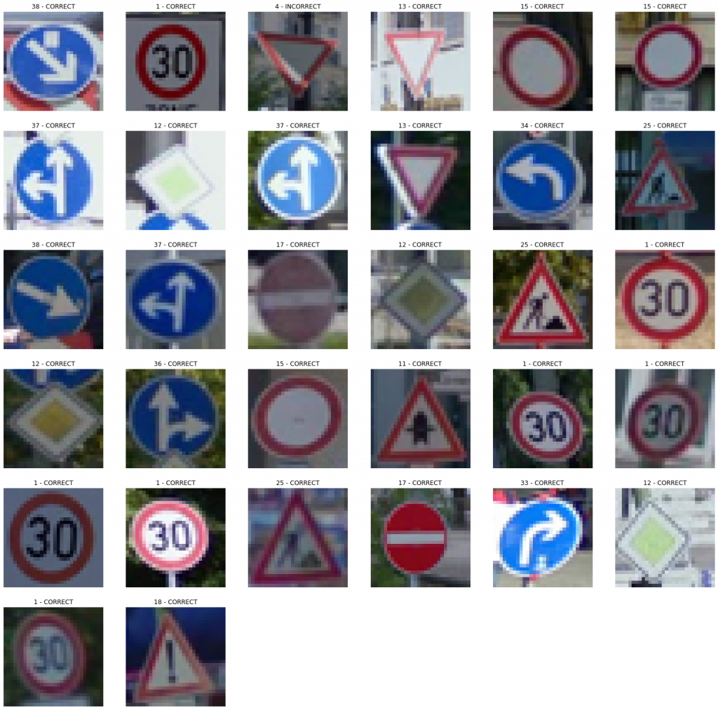
Again, it showed a similar accuracy for a completely unseen dataset. With a little bit of tweaking and troubleshooting, we should be able to improve the performances. But, let us focus on the enhancements on another day. For the moment, we are happy with the output produced by our model.
Do It Yourself!
Here, we will briefly explain how we build a simple, yet effective web application for testing the algorithm on the go. I think that the development of a web app might be beneficial because it showcases our capability to provide an end-to-end solution since we focus on the deployment process as well.
In the previous sections, we demonstrated how you can build a deep learning models from scratch, and test them against different datasets to measure the respective performances. However, we used the Jupyter Notebook interface to handle our coding experiments. We understand the difficulties posed by such an approach if you are a less tech-savvy person. Thus, we hereby present you a handy web application, where the trained models can be utilized by YOURSELF to experience how the models output results.
The application can be reached by visiting the following link, where the necessary instructions have been given for you to easily classify the traffic signs, YOURSELF! Enjoy!
Traffic Sign Recognizer | Do It Yourself!
Feature Additions
Detection of Unknown Images (From 12-07-2021 to 16-07-2021)
After the development of the web application, we realized that the application does not perform up to the expectations when it is presented with an image which does not consist of a trained traffic sign. Since the model had been instructed to strictly output only the designated traffic signs (43), the model was supposed to say that the submitted image belonged to the category of one of the trained traffic signs. This was a problem that we needed to address, and we followed a methodical approach to minimize the issues arising from our problematic approach.
Novelty/Anomaly detection is a research area, where different approaches have been suggested in the literature by the scholars to tackle the problem which we identified. One of the suggested approaches is to include an additional class to the existing list of classes by retraining the model with random images (non-traffic-sign images). Additionally, it is also suggested to create a binary model as a pre-filter which can classify the images by specifying whether the image is a traffic sign or not. For this approach as well, a set of random images are required for training purposes. If we are to follow a different approach, the option is to train a model using an object detection algorithm such as YOLO, and enhance the usability of the web application.
After considering the advantages and disadvantages of the different approaches mentioned above, it was decided to consider one of the first two approaches, because of the comparatively less effort needed to modify our existing model, while meeting our requirement. However, instead of singling out a particular approach, our intention was to implement a solution utilizing both approaches to increase eventual the user experience. As a result, a pre-filter was developed to create a binary classifier which essentially classifies whether an image is a traffic sign or not. After the binary classification, the images are sent through the usual multi-class classifier where the classifier contains an additional class called “Unknown Traffic Sign” to denote images which do not adhere to the characteristics of a trained traffic sign. The following figure illustrates the proposed combined approach.
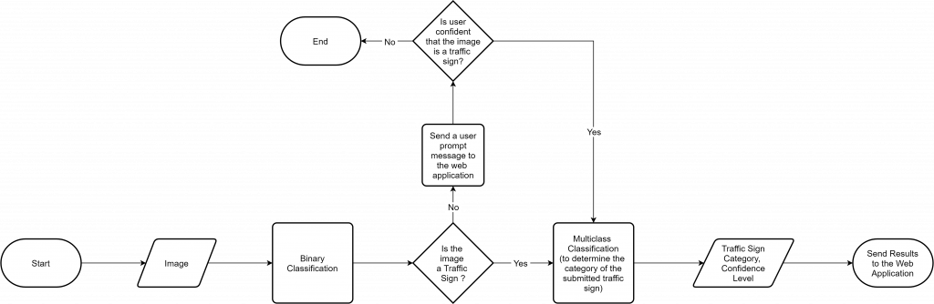
In order to implement the workflow given in the above figure, the following changes were applied.
Adding “Unknown Traffic Sign” to the existing model
- This process increased the number of classes from 43 to 44.
- To achieve this task, 1930 more random images were added from the COCO Dataset to our training distribution, and assigned the new class label (44: Unknown Traffic Sign) accordingly.
- At the same time, 615 images from the COCO Dataset, were added to the Test dataset.
- The same NN architecture that we had used earlier, was utilized with an additional output class, and the model was retrained to achieve a classification accuracy of 99.57% for the validation dataset.
- The model performed well by minimizing the issues that existed with the recognition of non-traffic-signs.
Development of a binary classifier as a pre-filter
- This process entails the development of a binary classifier which classifies whether an image is a traffic sign or not.
- For this purpose, all the images from the GTSRB Traffic Sign dataset (51,839 images) were considered along with 45,670 images from the COCO dataset (non-traffic-signs).
- Necessary splits and preprocessing tasks were applied before the training process.
- Improved the model iteratively (as we had done in the previous version) to create the binary classifier.
- Managed to achieve a validation accuracy of 99.81% and an accuracy of 99.72% for the left-out Test dataset.
Integration
- As elaborated in the above figure, a submitted image first goes through the binary classifier to detect whether the image is a traffic sign or not. If it is detected as a valid traffic sign, the image will be checked by the traffic sign classifier, and a suitable feedback is sent back to the frontend.
- If the submitted image is detected as a non-traffic-sign image, the user is prompted with a message, and the user confirmation is required to proceed further (to force the application to classify the image regardless of its type).
- If the user wishes to proceed, the image is sent
Selecting between PoCs, Prototypes, and MVPs.

Many companies struggle to choose the aptest technique to validate their concept and choose between POC, Prototypes, and MVP. In our previous context, we discussed the definitions, applications, advantages, and use cases of these elements. You can find the link to the article here and peruse the write-up for a comprehensive understanding.
It is essential to know that it depends on the business idea or the end product and your target audience (B2B, or B2C, B2B2C); and you may need to use PoC, Prototype, MVP or a combination accordingly.
Idea validation using these concepts will ensure that your final product will enable you to achieve its ultimate goal.
A PoC can usually provide a direct response to whether the concept will be viable or not for the target audience. Idea feasibility will be measured here, and with the comeback, you can decide whether to proceed with the existing plan or not. Furthermore, a PoC can help convince your initial pre-seed investors that your concept can be implemented and is technically viable.
On the other hand, MVP enables companies to grasp information about the target user's experience and respond to the core business purpose of the application. The insights received from actual users helps to validate the overall objectives, identify the user pain points, and address the issues over time.
If you want to present how exactly your final product will look like, or manifest the main design elements, prototyping is the best way to give the big picture to the end user. It further helps to run multiple test areas while saving your resources. If you are looking for investors to work on your project, a tested prototype is the best way to demonstrate and pitch your product.
Should PoC, Prototype, and MVP be Throwaway Builds (Minimum Initial Investment)
It is always better to look at PoC and MVP as throwaway codes. If your business idea takes momentum and finds traction, it is vital to build everything from scratch with architecture and design to cope with it for the next 3 to 5 years.
For PoC, think of the least expensive way to implement. Typically, when developing a PoC, factors like product scale, architecture, UI elements are not considered. Instead, the requirement is to check on technical feasibility and customer feedback on your new product idea or a particular feature.
With all things considered, your PoC will be a hardly scalable piece to turn out for something decent. Hence, it is better to consider it as a throwaway build.
In relation to prototyping, it can be either a throwaway or a part of your final user interface, depending on the model type you select. For example, you can use rapid throwaway prototypes to receive user feedback and discard it later. These models are used to validate the system functionalities and requirements. Hence, it needs to be removed as it does not add any advantage to the final UX/UI elements.
For MVP, you may have to build in a way that could cope up with the demand for the next 12 to 18 months (Not a rule of thumb, but empirically proven ). It is common to see startups control the growth without hurting long term plans to build the post MVP version. However, for the long run, it is essential to opt for a complete rewrite ensuring your final product can have flexibility, extensibility and adaptation with upcoming technology and supplementary changes.
A Guide to Choose from Poc, Prototype, and MVP
Exhibiting a decision matrix using a table. - includes questions and scores for users to choose the correct method for their products.
Check out the reference tables at the end of this article.
Decision Matrix
| Parameters | POC | Prototype | MVP |
| Use Case | For Technology/Market/Behavior disruption (completely new idea, so need to prove a concept is viable to build) | To verify user journeys and messaging in a solution are understood by the intended users. Save time and money. Could used to attract seed funding | Get actual users to use your solution to solve the identified problem. Evaluating your solution solves the problem in an acceptable manner. Gather feedback from users to improve upcoming versions of the solution. Aim to the initial target audience response |
| Purpose | To verify technical/market/behavioral assumptions before getting down to development. / To clarify which way to go with the development. Convince internal stakeholders | Make the application usable for its intended users. To assure that the end users could navigate and get the job done using the solution. It is the working model of several aspects of your product. Prototypes help make decisions about product development and reduce the no. of mistakes and waste. | To prove, your solution is effectively solving a problem and it is effective enough for the customer to pay for solution.To get the minimum version of the product to the market |
| Form of implementation | Most rudimentary implementation to prove the relevant disruption is viable to implement | High or Low fidelity Wireframes/UI, users could navigate through different screens but nothing has been implemented | Usable solution by its real user, just to solve the identified problem (nothing more, nothing less) |
| Target audience | Internal users (Decision makers about the project GO/NO GO) | Specifically selected sample of target audience (real users). Should be able to access more than once to verify the prototypes (should be able to involve with iterative process of prototype building) | Sample of target audience. Easily accessible, Give genuine feedback. Test the product with a pre-selected potential customer group |
| Cost | Less budget and is ideal to collect internal funding. Might have to invest on new tools and accessories. | Much less cost to build the prototype compared to PoC or MVP. More time/resources spent here saves time/resource at the expensive development phase | No compromise on quality as the end product would be used by real users. Cut the cost by reducing features, not the quality. Well-defined budgets and looks for investment |
| Human Resources | Requires technical experts to develop the basic concept. Could involve tech related R&D | Less technical resources as no coding / development is involved. Need to recruit testers, Iterative design processes | Here you are developing the actual product (at a smaller scale with less features) So needs full technical expertise |
| Risk Evaluation | PoC involves the highest risk or all. But lessen the risk in upcoming phases. | Reduce the risk in terms of user satisfaction in product navigation | Reduce the risk of losing time and resources of the full scale development |
| User Interaction | N/A since is its used internally | Gives an overview to the end user how the end product will look like with basic elements and navigation. Highly interactive with users but without real functionality. | Full user interaction. UI/UX, Key Functions and even feedback from users also a part of interaction |
| Apparent time to create | If you have several options or if you uncertain about the feasibility of the concept | When you are confident about your idea and needs to start and test the design process | When you are positive about the idea and the design, and ready to launch it to the market |
| When to Show the investors | Pre-seed / Seed | Pre-seed / Seed | Pre-seed, Seed, rarely for Round A |
| Cashflow | Negative (expenses only) | Could leads to Positive cash flows from Investors (Seed level) | Should lead to Positive cash flows from service revenues & Investors |
| Extended use | Can be used to develop MVP | Output can be used to develop the solution. No waste. If the prototype consist of UI design, it could be used for the development | Can be expanded and used for the full version of the product. You may have to throw away the code (Do not hesitate to do so) |
| What you should not do? | Invest time/resources to make the PoC usable to others.Implement things that have been already proven | Use placeholder content or graphics. Train/Assist testers. Test how UI/UX work on real environment | Compromise on quality Implement extra/supplementary features |
| Outsource or in-house work | At this stage, you are working on an idea to check out its possibilities of turning it into reality. Hence, it is ideal to do in-house to ensure that your concept would not be revealed to third parties /competitors. | Prototypes can be fully outsourced as they will be exposed to the public for test-run purposes. | MVP can be done internally or with the contribution of a third party. A mixed team is preferred here to build up the product. Here, the expertise (outsource party) can help with the best techniques while the in-house team is conscious of the progress/development plan. |
Final Take Away
Building a solid foundation is essential to deliver a successful software product. Your PoC, prototypes, and MVP will be your foundation for the process, with actual feedback. They will help you to iterate the product process and enhance the features to meet the user requirements or the ‘real-needs’.
However, software product development is not limited to paying attention only to the initial process but is involved with many crucial steps that need to be considered throughout the proceeding. With that note, the next phase of the development process will be discussed in future articles.